mathr / blog / #

This all started when I was trying to add 3D sound to the reboot of Interstellar Interference. I found some HRIRs (head-related impulse responses), and I encoded the 3D sources into 1st-order ambisonics, then decoded the ambisonics to virtual speaker locations corresponding to each HRIR and convolved. But it was epicly slow (220x slower than realtime), and didn't even sound very good, so I thought about modelling the head in a less brute-force way.

So the problem became, given a source location relative to the oriented head, find a simple filter that makes the far ear quieter than the near ear, taking into account diffraction (low frequencies are shadowed much less than high frequencies). I implemented the wave equation in a couple of OpenGL shaders using Fragmentarium (a simple GLSL IDE), and got some response curves for frequencies spaced every octave from about 75Hz to 4.8kHz. But I also was intrigued by the interference between the reflections from the edge of the screen, and that got me thinking about resonant modes in acoustics.

The wave equation simulation I made needed about 50k iterations to get a result for a single frequency, taking long enough to get annoying. The wave equation constrains a function \(F\) of time and space like this:

\[ \frac{\partial^2}{{\partial t}^2} F = c^2 \frac{\partial^2}{{\partial x}^2} F \]

where \(c\) is the speed of sound. Apparently some separation of variables technique that I didn't quite understand can be applied, which gives an equation that doesn't depend on time:

\[ \frac{\partial^2}{{\partial x}^2} F = -\left(\frac{\omega}{c}\right)^2 F \]

where \(\omega\) is the angular frequency of the wave. This made me think of eigensystems, which have:

\[ M v = \lambda v \]

where typically \(M\) is a matrix, \(v\) is a vector, and \(\lambda\) is a scalar. The solutions are pairs \((\lambda, v)\) of eigenvalues and eigenvectors.

So I needed to turn the partial differential into a matrix, which is conceptually not too hard, but the implementation was a little grotty. In 1D, one can approximate like this (up to a factor of \(h\) or \(h^2\) or something, which turns out to be irrelevant for the purposes of this post):

\[ \frac{\partial^2}{{\partial x}^2} F \approx F(x-h) - 2 F(x) + F(x + h)\]

where \(h\) is the distance between cells of a discrete mesh approximating the contiuum. Modelling \(F\) as a 1D vector, this gives a matrix like:

\[ \left( \begin{array}{rrrr} \ddots & & & \\ 1 & -2 & 1 & \\ & 1 & -2 & 1 \\ & & & \ddots \end{array} \right) \]

with all the \(-2\) along the main diagonal. This doesn't take into account what happens at the ends of the mesh, to make \(F\) be zero there I set the top-left-most and bottom-right-most value to 1 (all the elements are zero unless otherwise specified - leaving a blank space is easier to read). In 2D, the stencil for a single point (previously \((1, -2, 1)\) in 1D) now looks like this:

\[ \left( \begin{array}{rrr} & 1 & \\ 1 & -4 & 1 \\ & 1 & \end{array} \right) \]

But we have to unwrap the 2D grid into a 1D vector, and make a 2D matrix (as before) to solve for eigenvalues and eigenvectors. With the same boundary conditions as before, here's what the resulting \(16 \times 16\) matrix looks like for a \(4 \times 4\) grid:

\[ \left( \begin{array}{rrrrrrrrrrrrrrrr} 1 & & & & & & & & & & & & & & & \\ & 1 & & & & & & & & & & & & & & \\ & & 1 & & & & & & & & & & & & & \\ & & & 1 & & & & & & & & & & & & \\ & & & & 1 & & & & & & & & & & & \\ & 1 & & & 1 & -4 & 1 & & & 1 & & & & & & \\ & & 1 & & & 1 & -4 & 1 & & & 1 & & & & & \\ & & & & & & & 1 & & & & & & & & \\ & & & & & & & & 1 & & & & & & & \\ & & & & & 1 & & & 1 & -4 & 1 & & & 1 & & \\ & & & & & & 1 & & & 1 & -4 & 1 & & & 1 & \\ & & & & & & & & & & & 1 & & & & \\ & & & & & & & & & & & & 1 & & & \\ & & & & & & & & & & & & & 1 & & \\ & & & & & & & & & & & & & & 1 & \\ & & & & & & & & & & & & & & & 1 \end{array} \right) \]

As you can see, it's pretty sparse, with very few non-zero values. Solving eigensystems is not exactly trivial, but luckily several good free software packages provide well-tested implementations. I used GNU Octave, which has two key functions: spconvert takes a dense matrix representation of a sparse matrix and builds a sparse matrix, and eigs solves the sparse eigensystem - I chose to let it find the 35 smallest-magnitude eigenvalues and their corresponding eigenvectors, which correspond to the lowest-frequency modes.

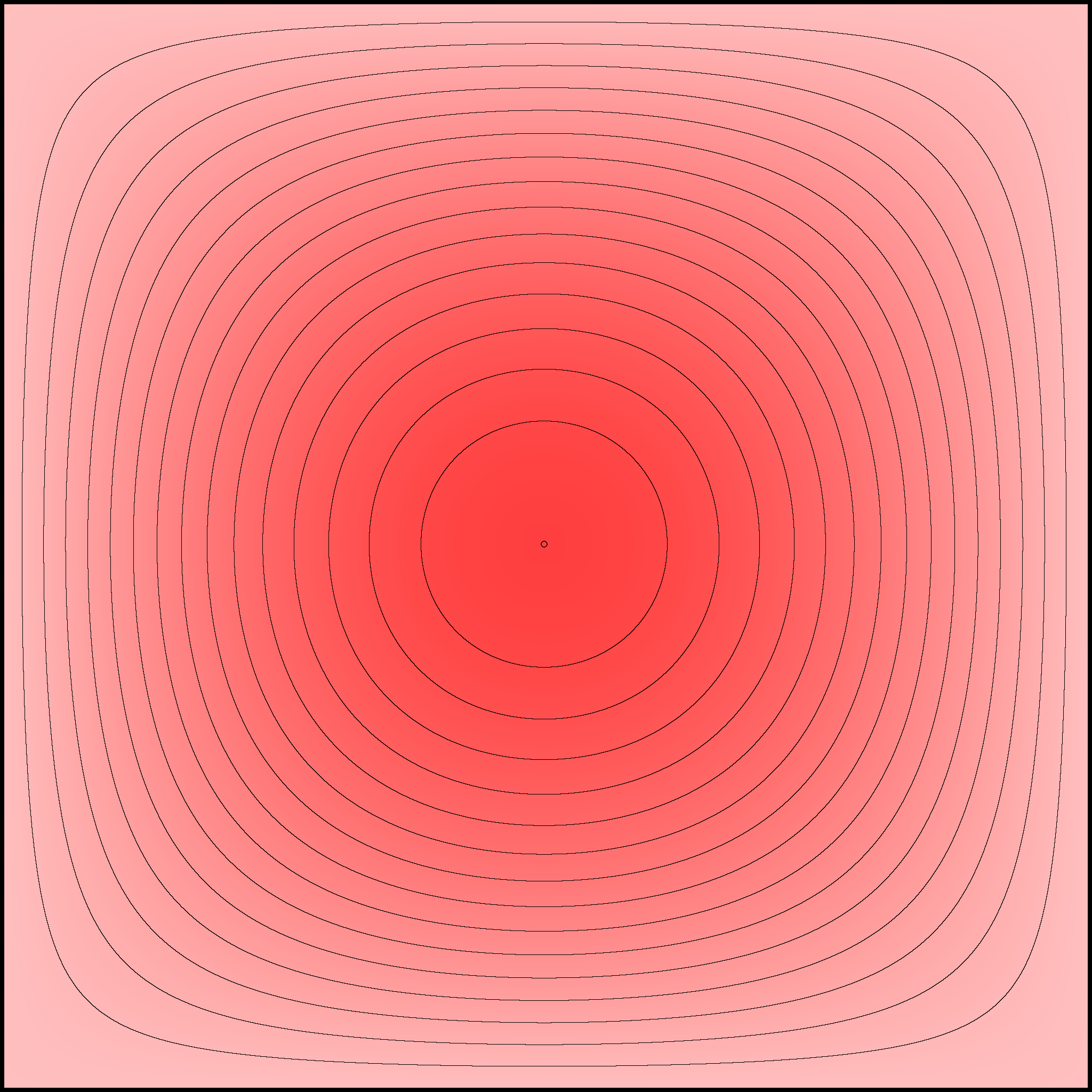
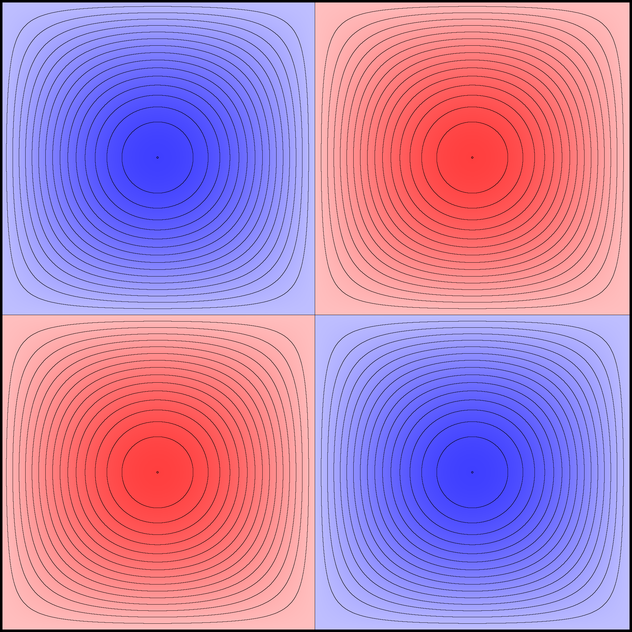
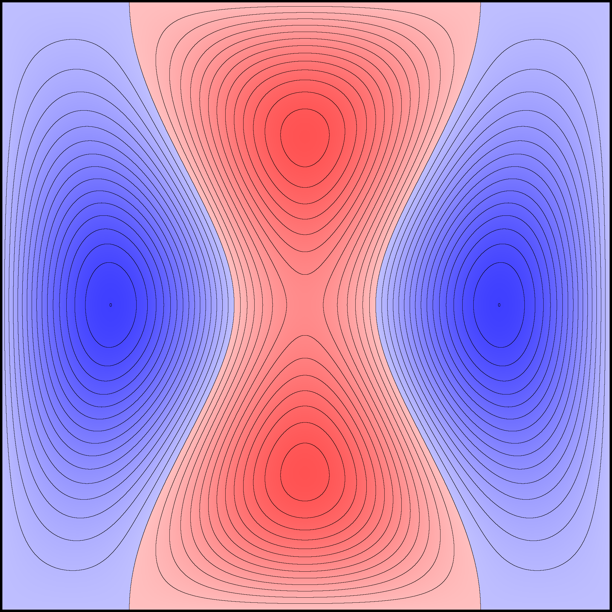
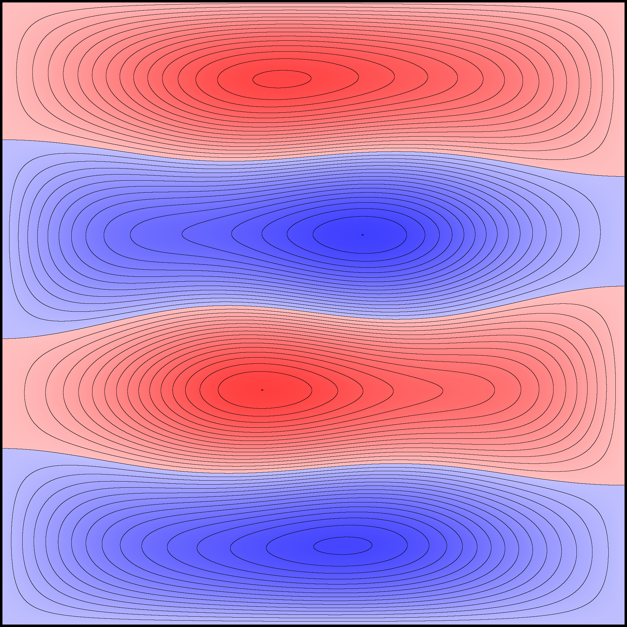
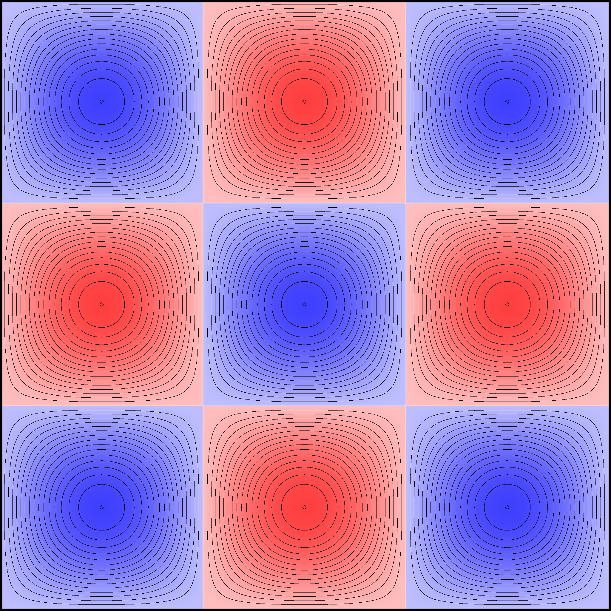
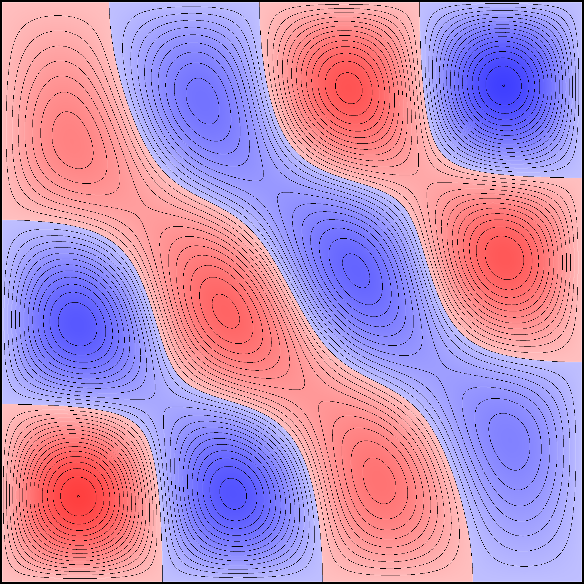
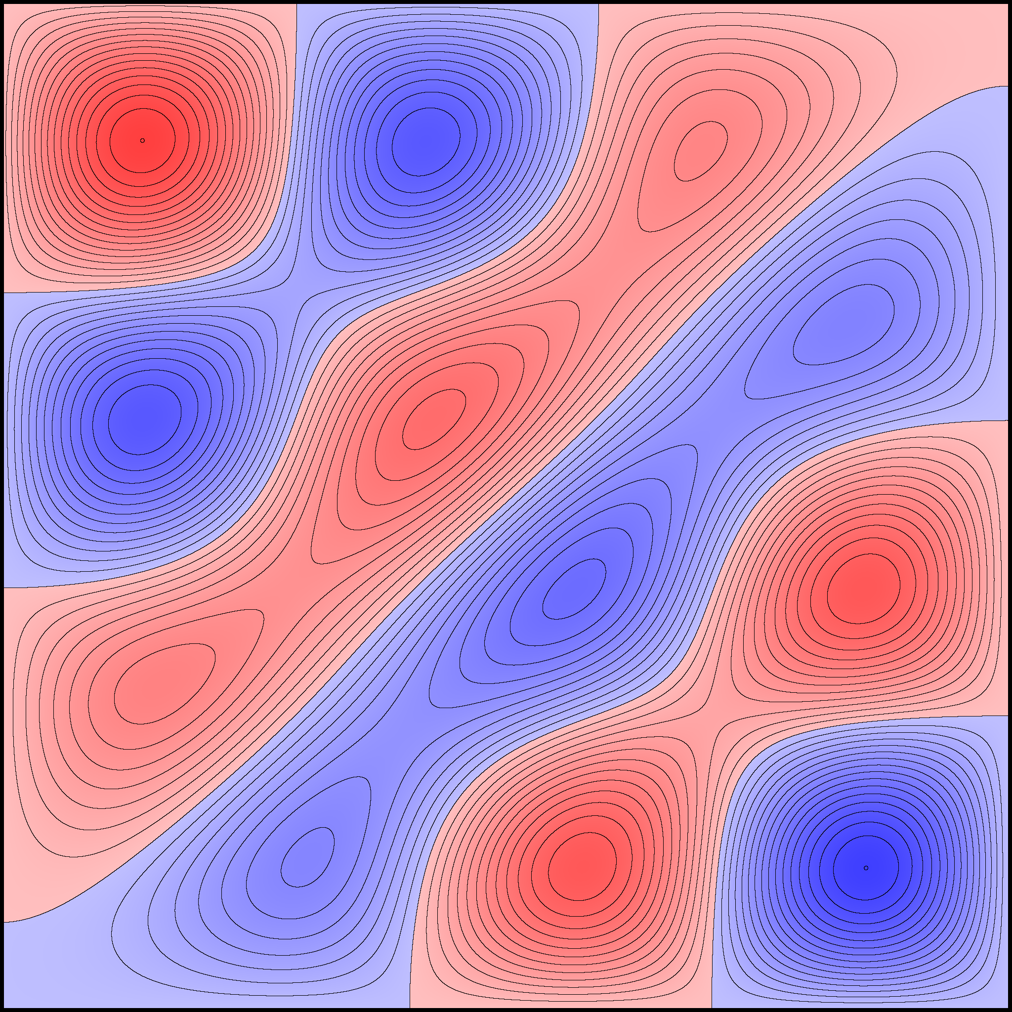
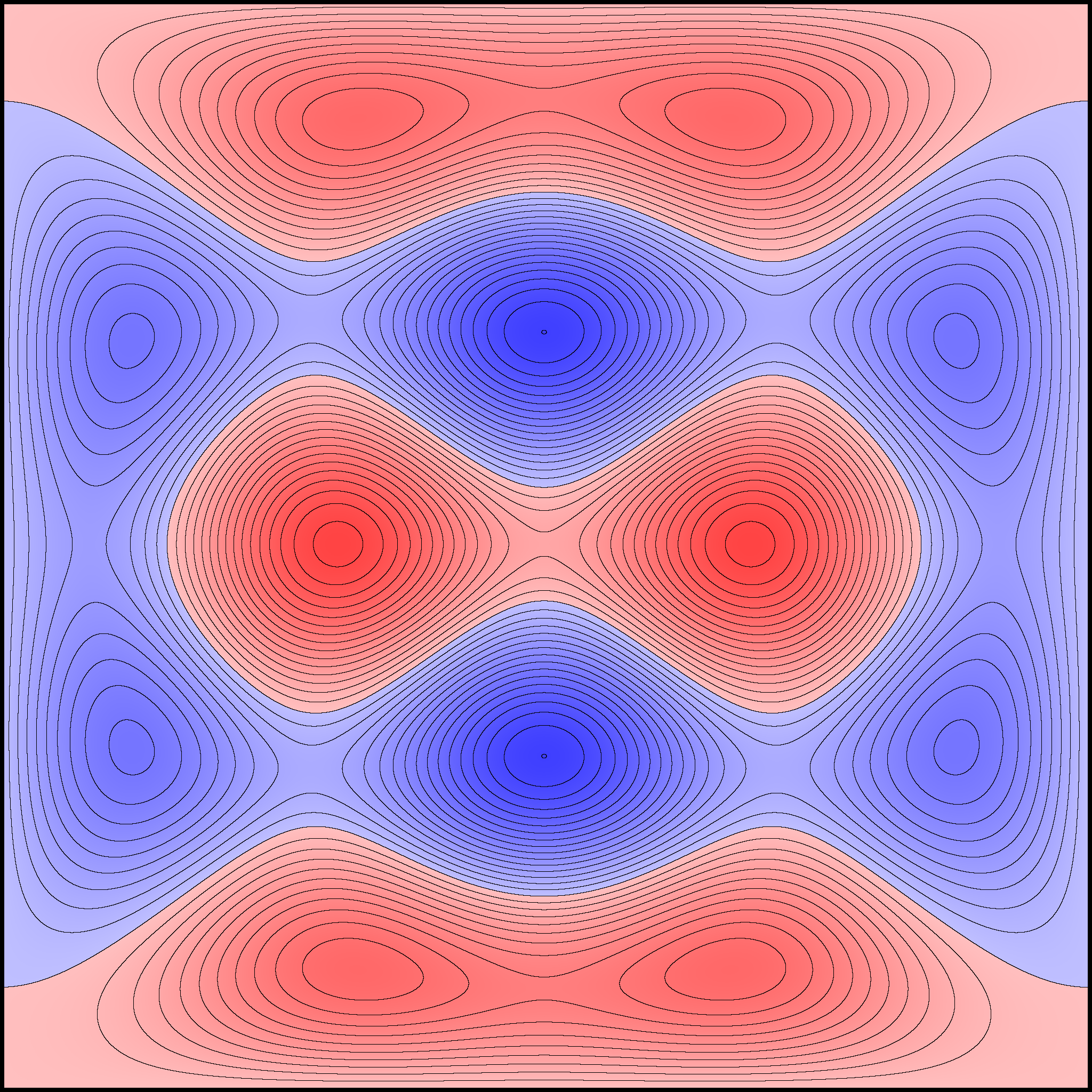
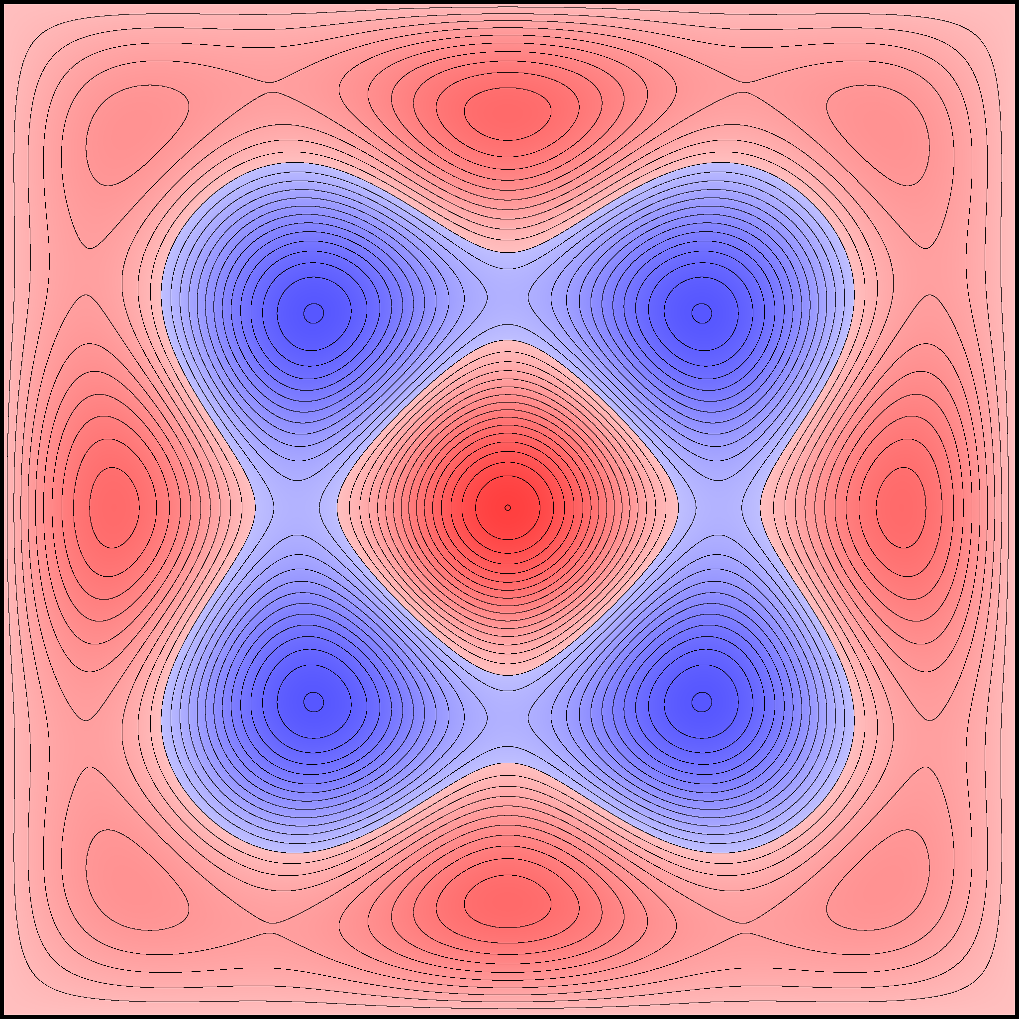
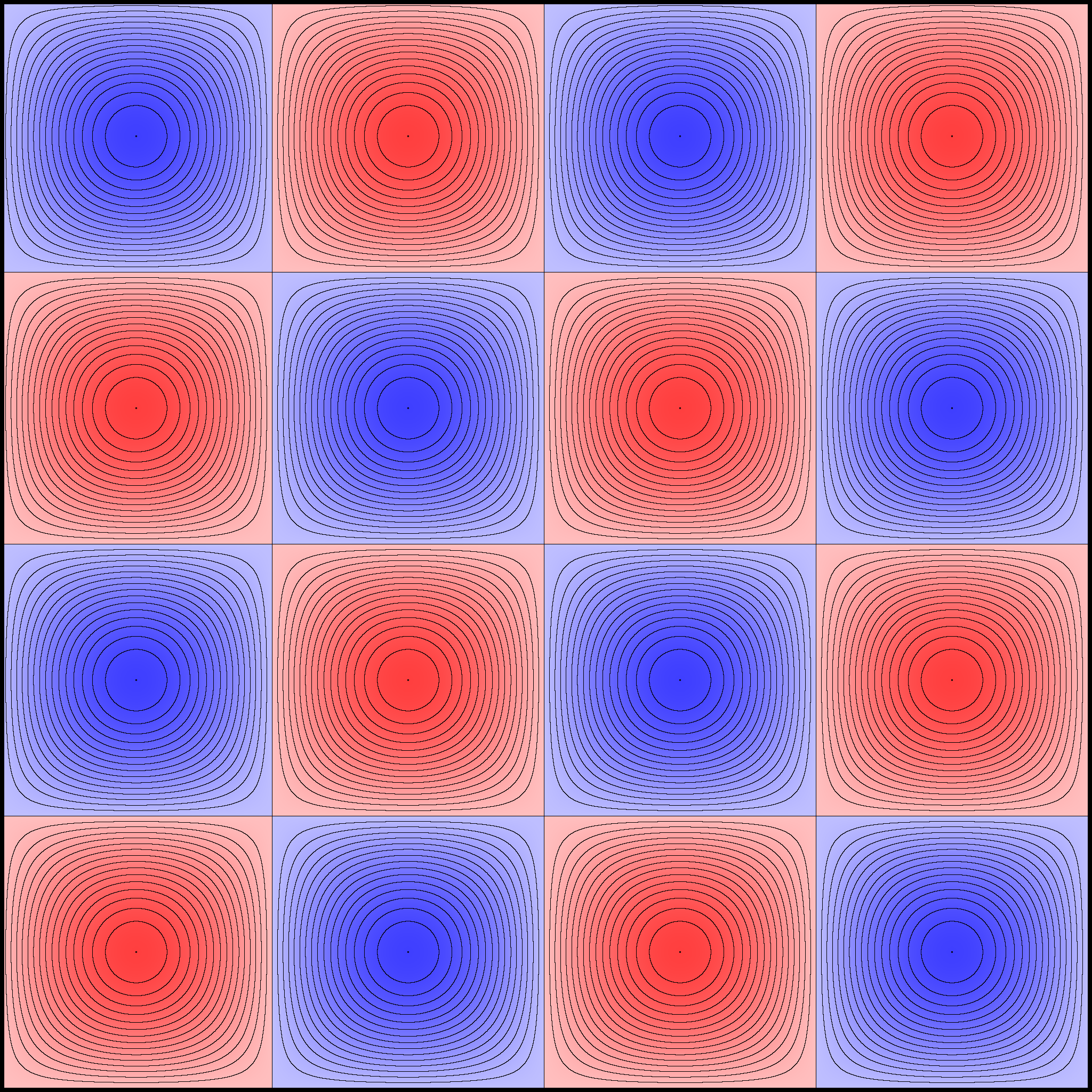
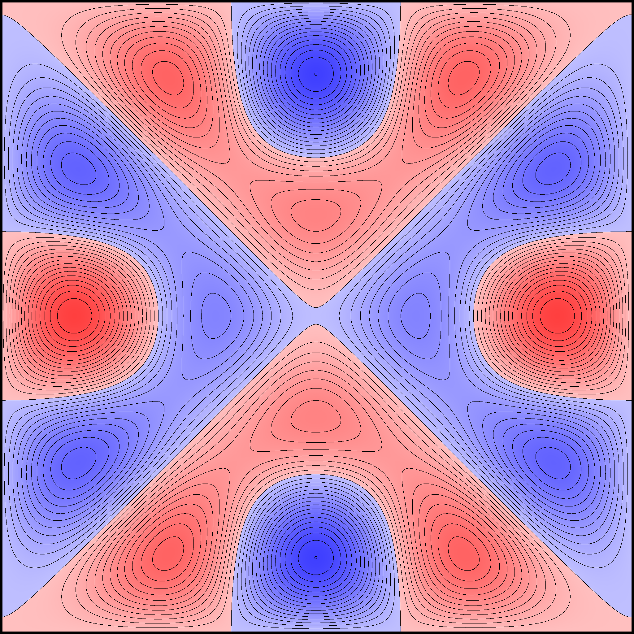
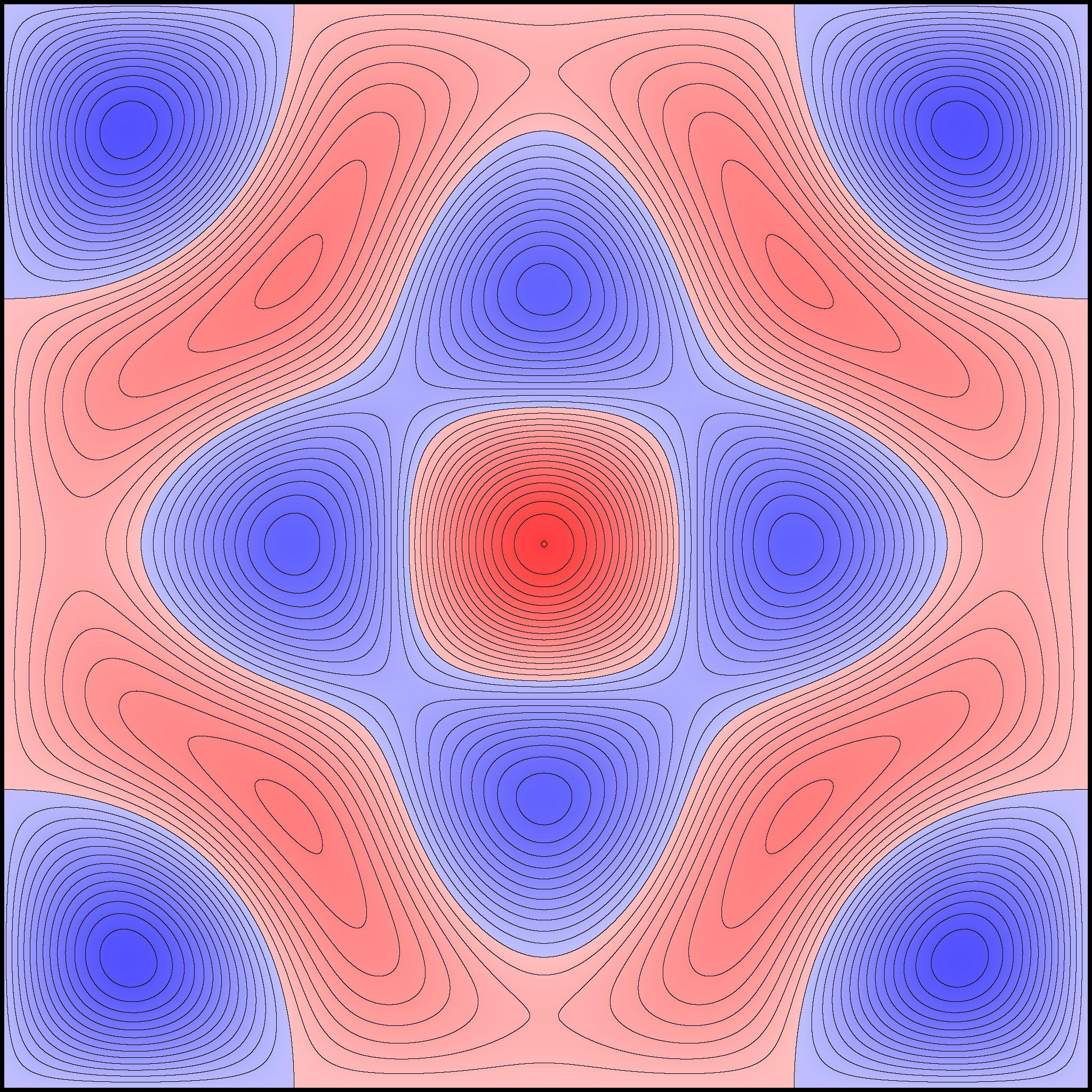
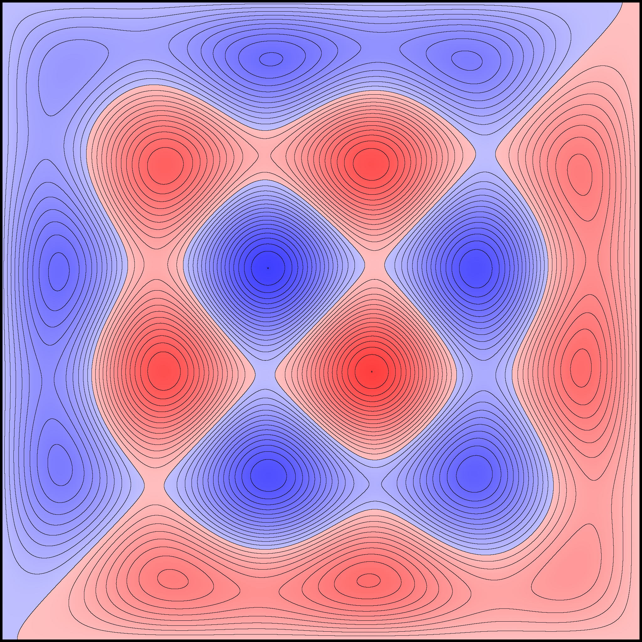
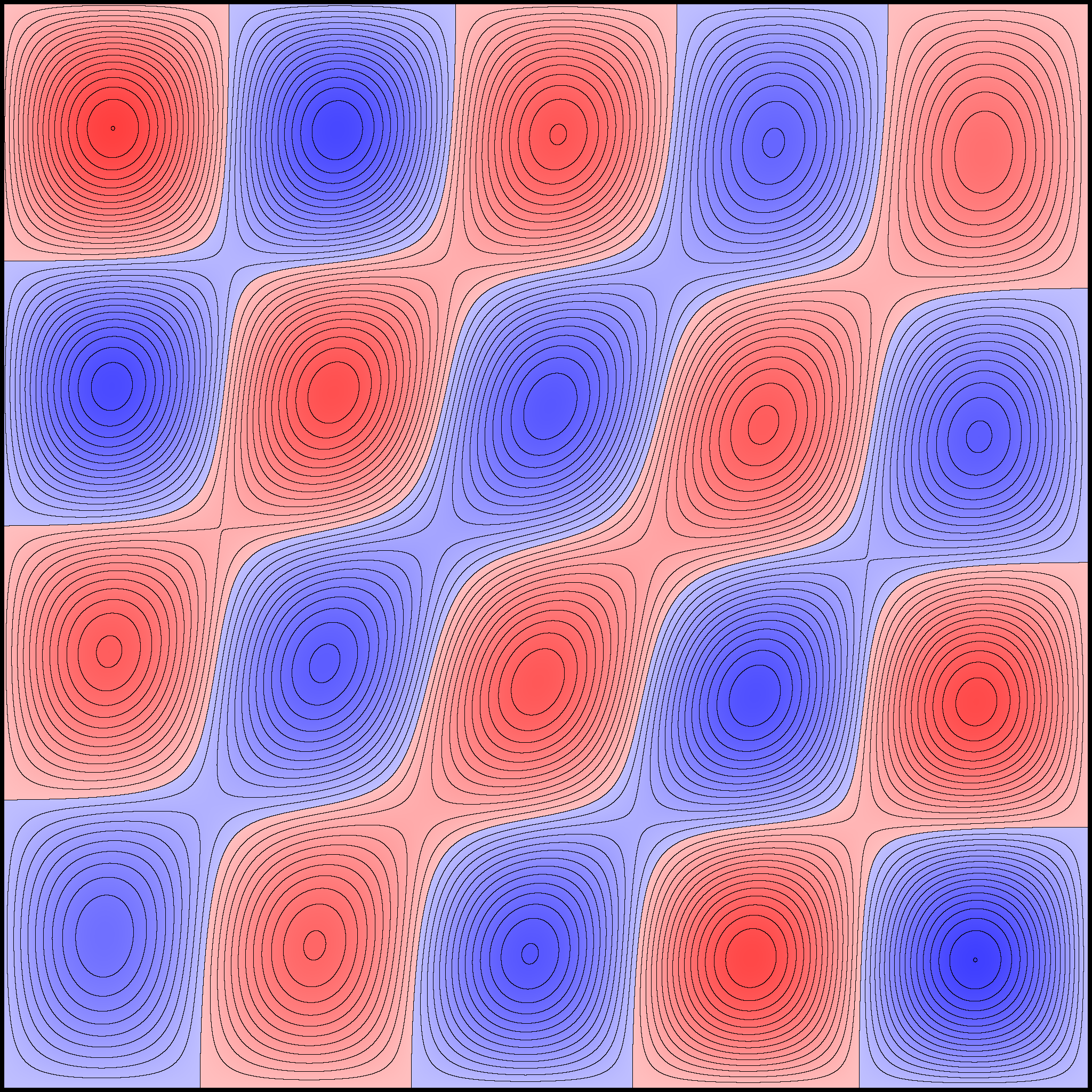
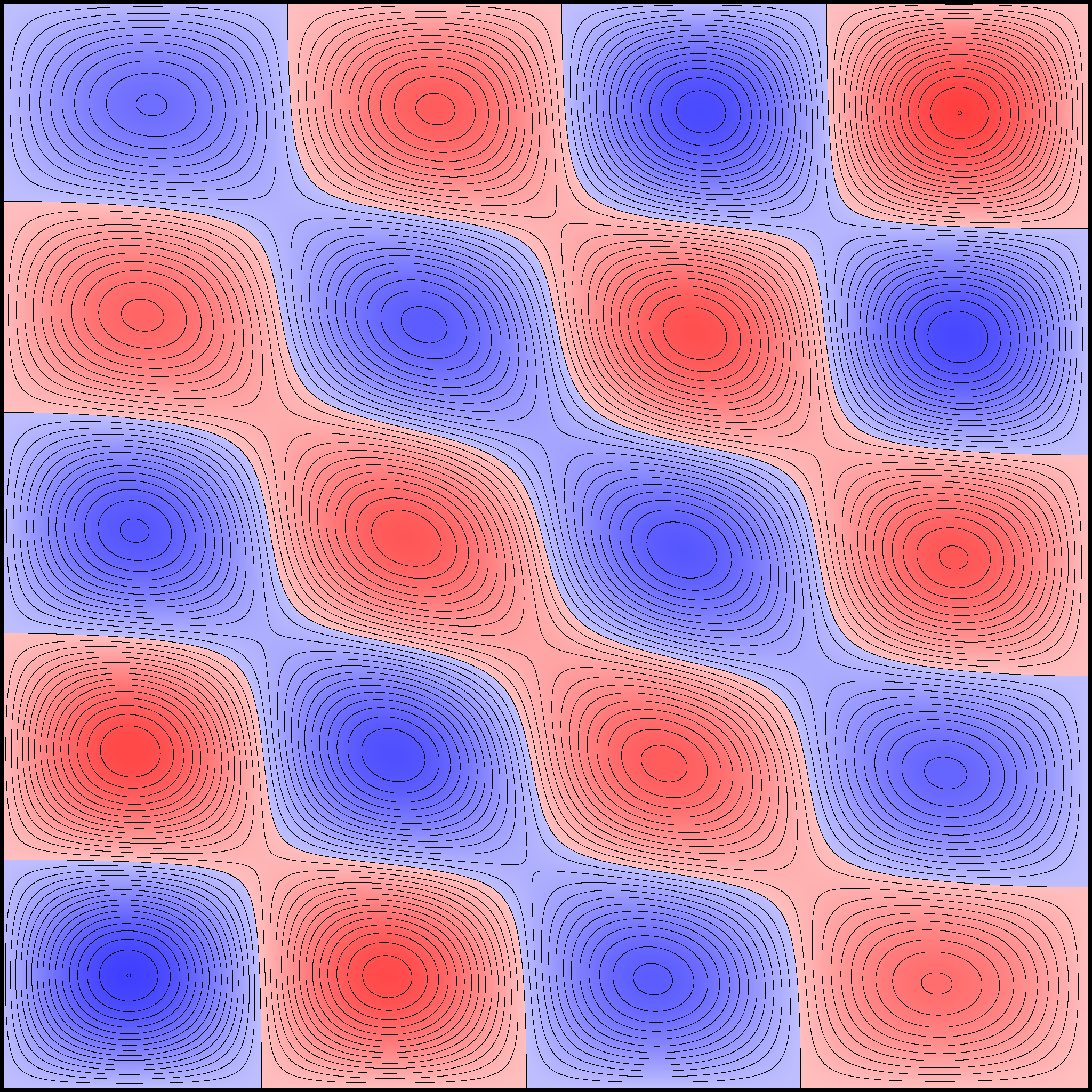
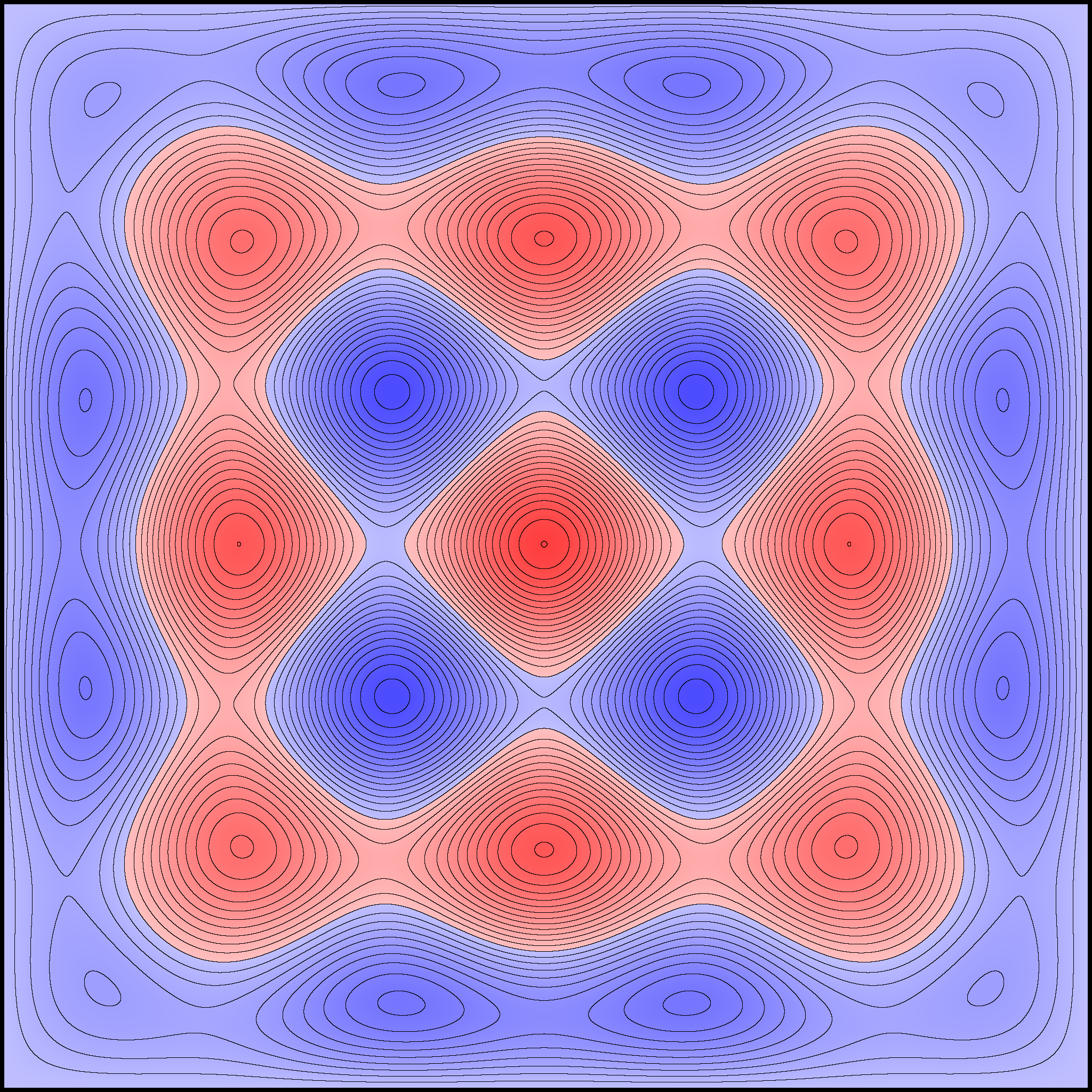
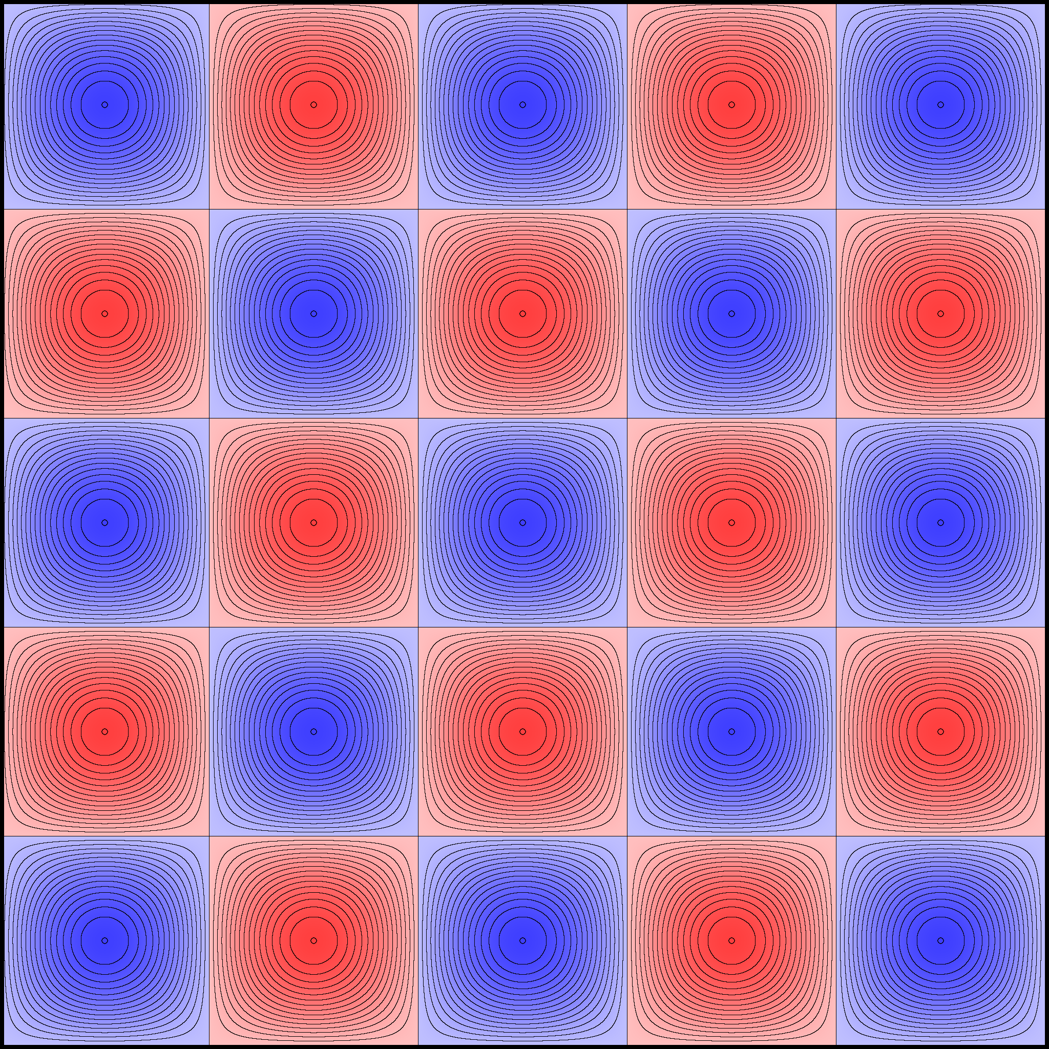
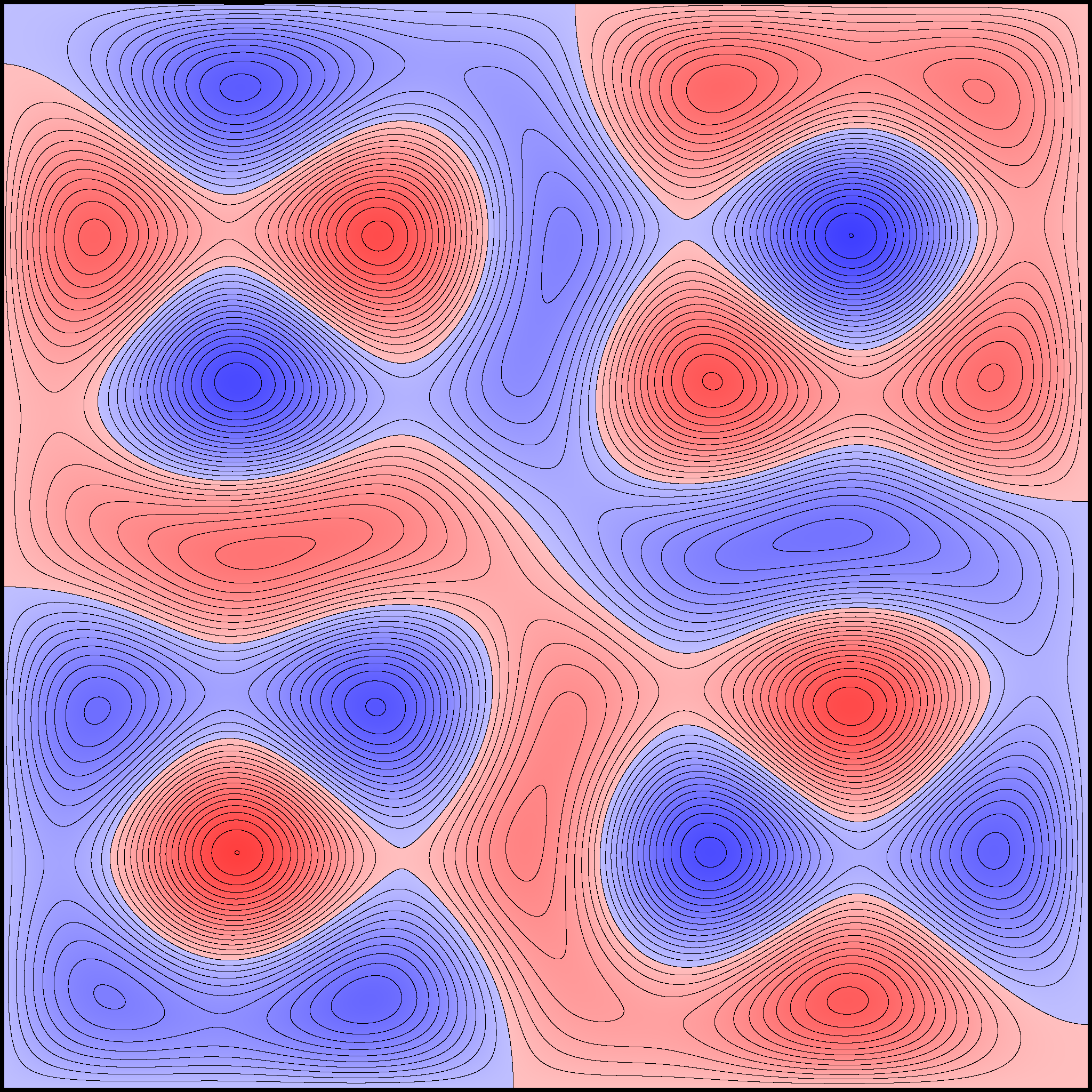
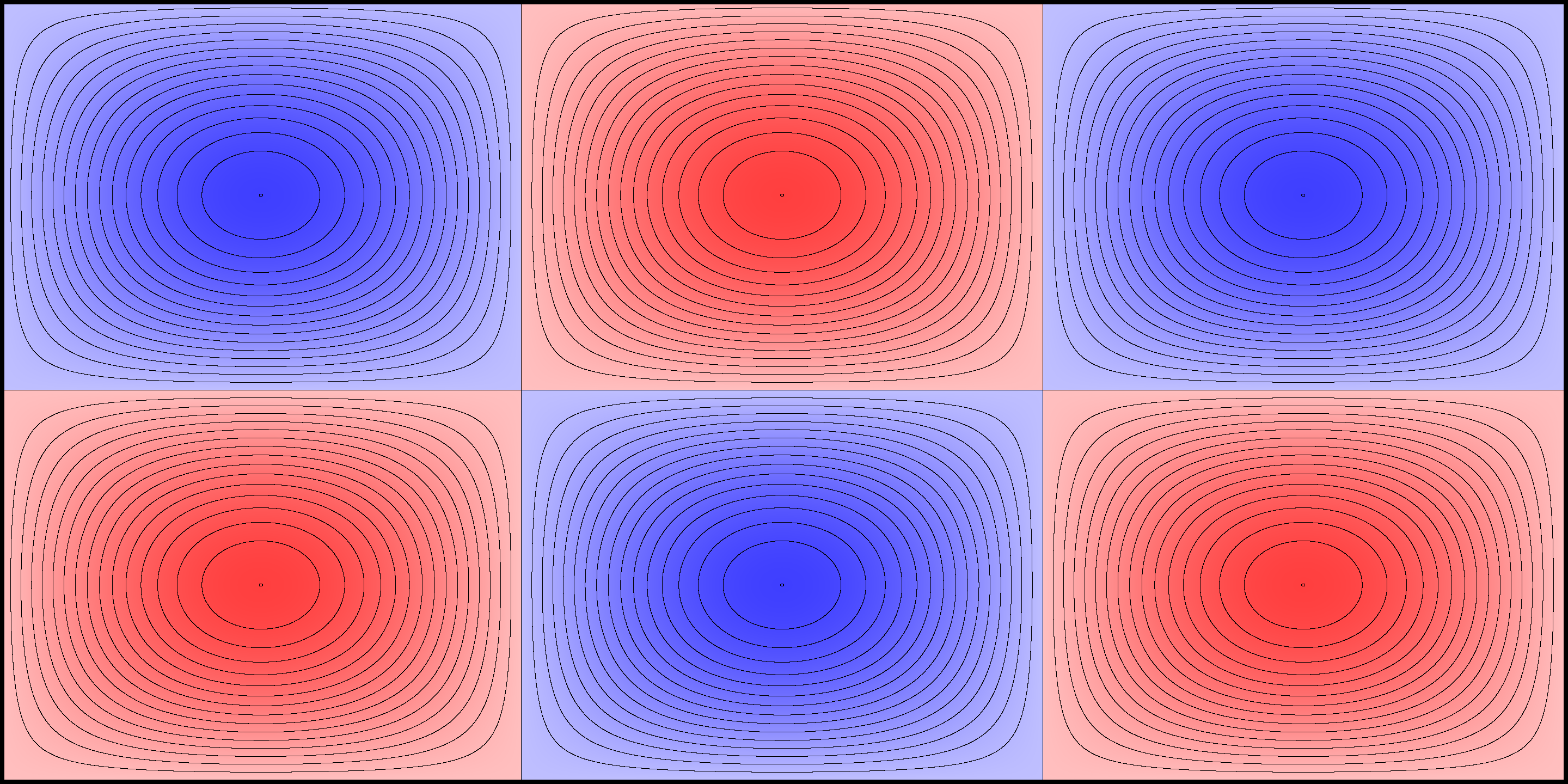
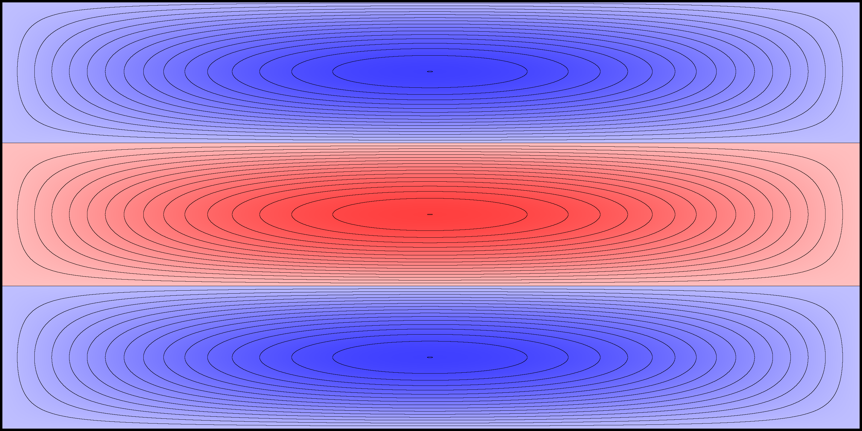
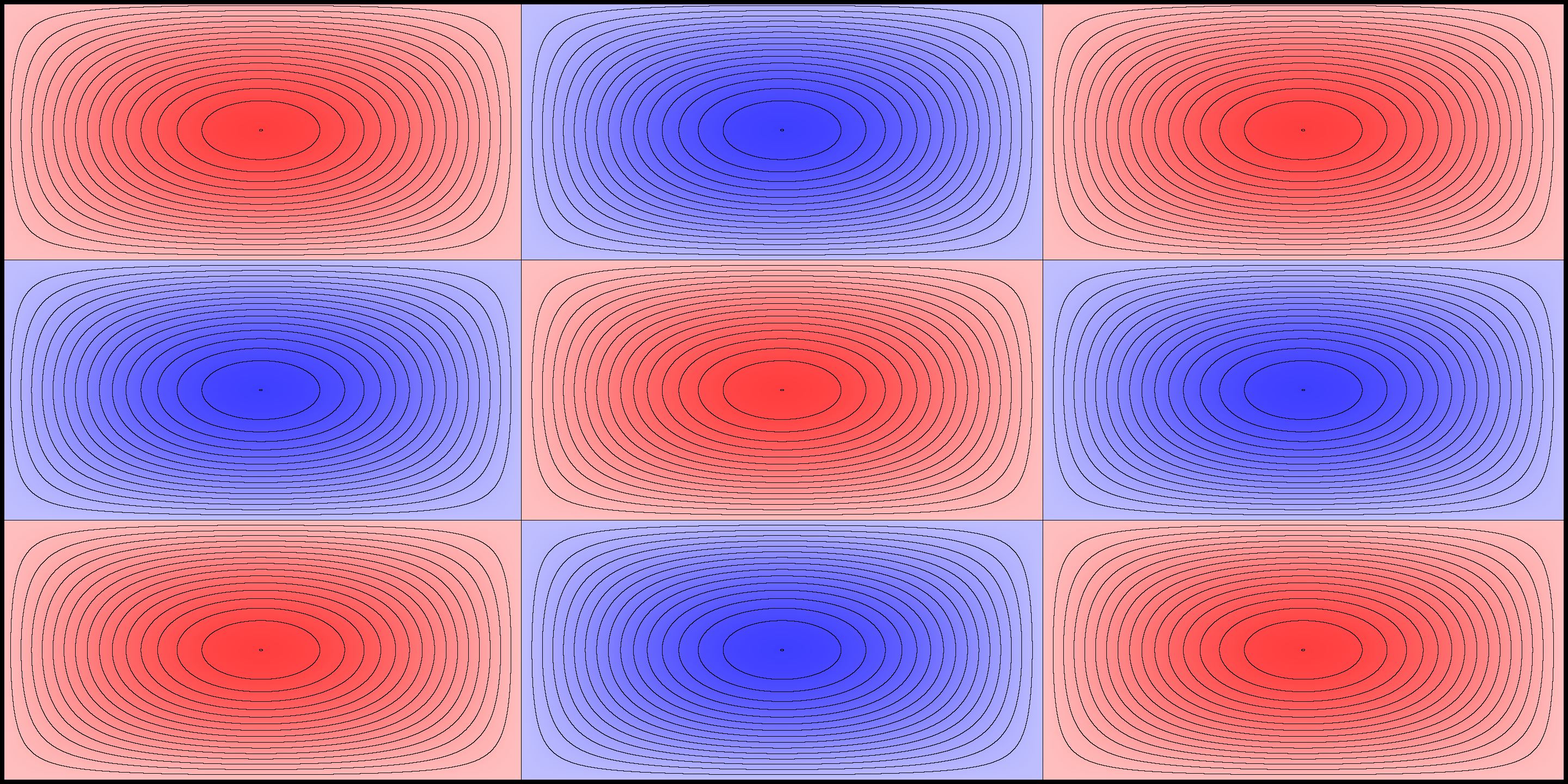
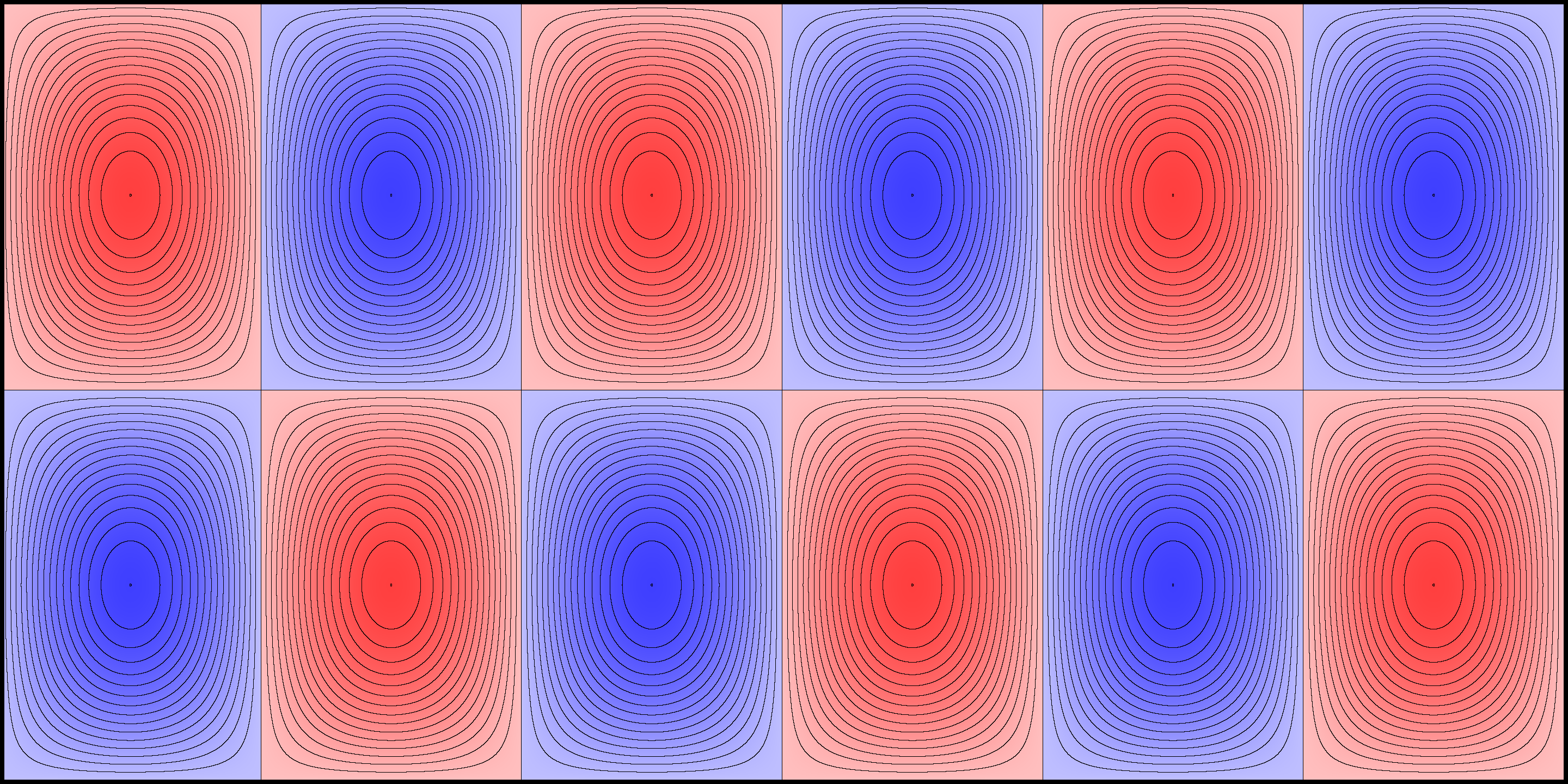
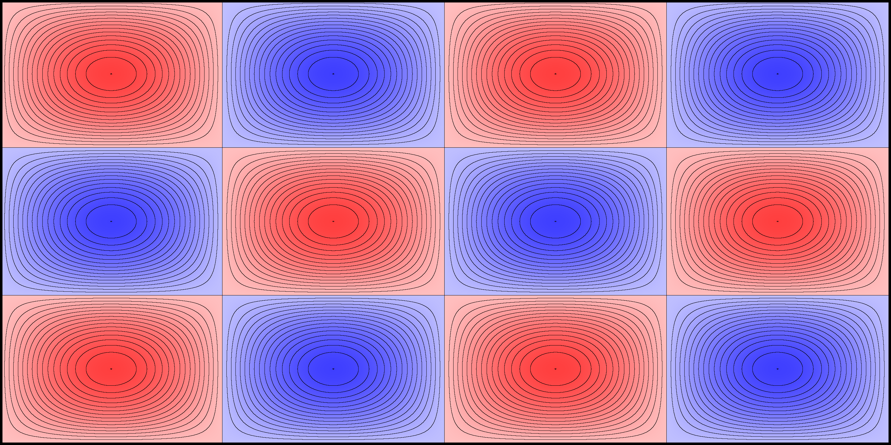
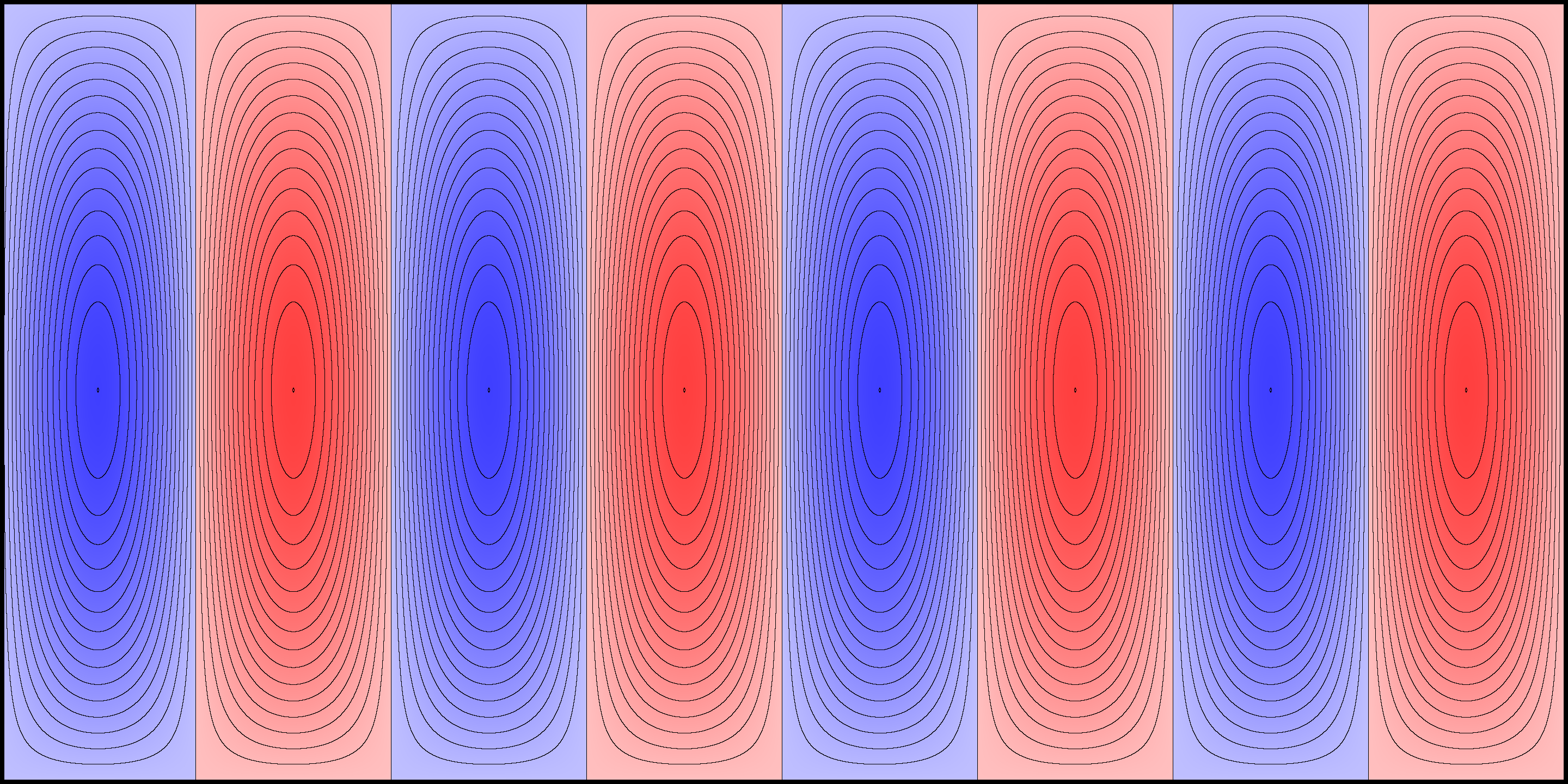
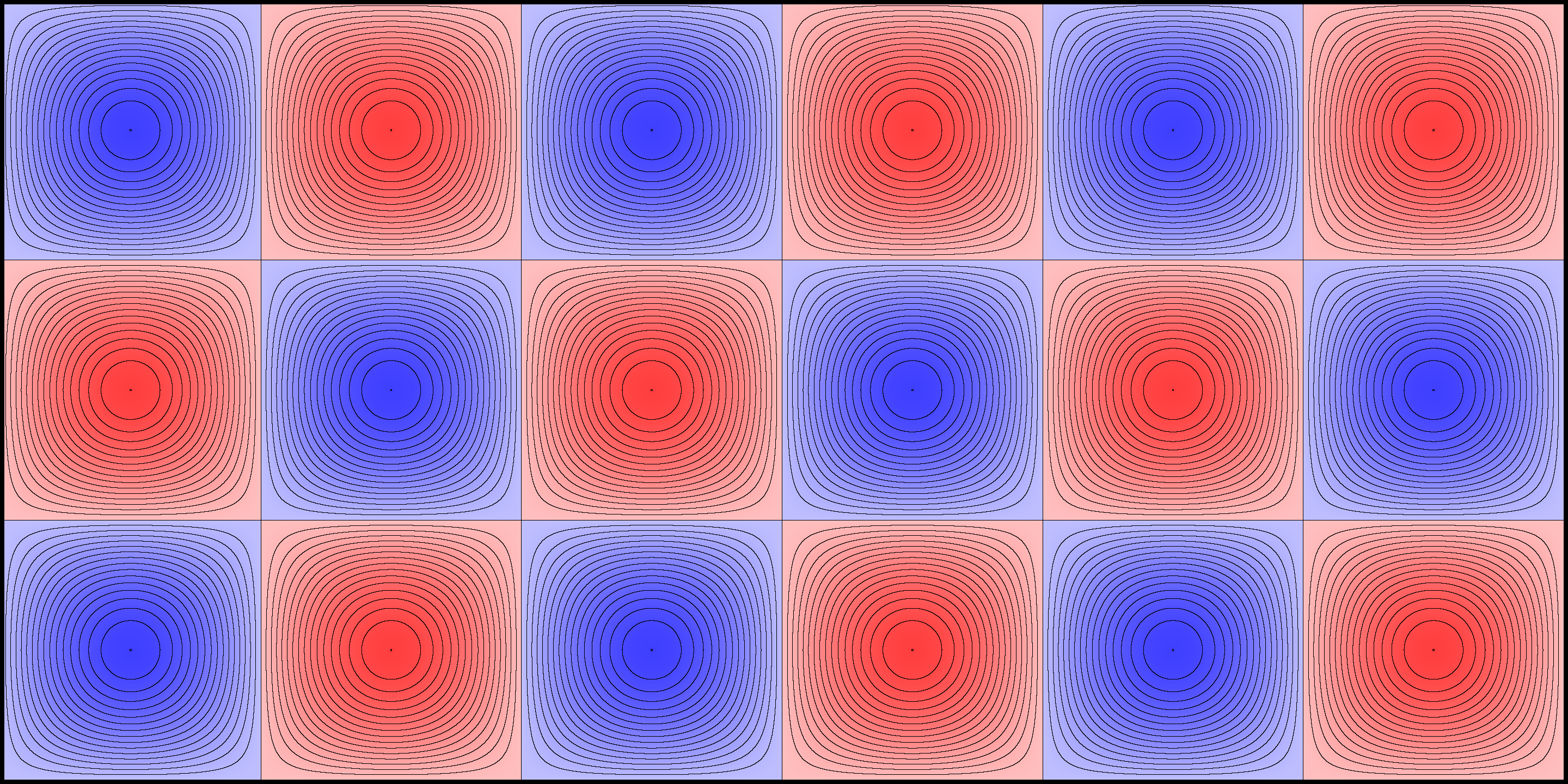
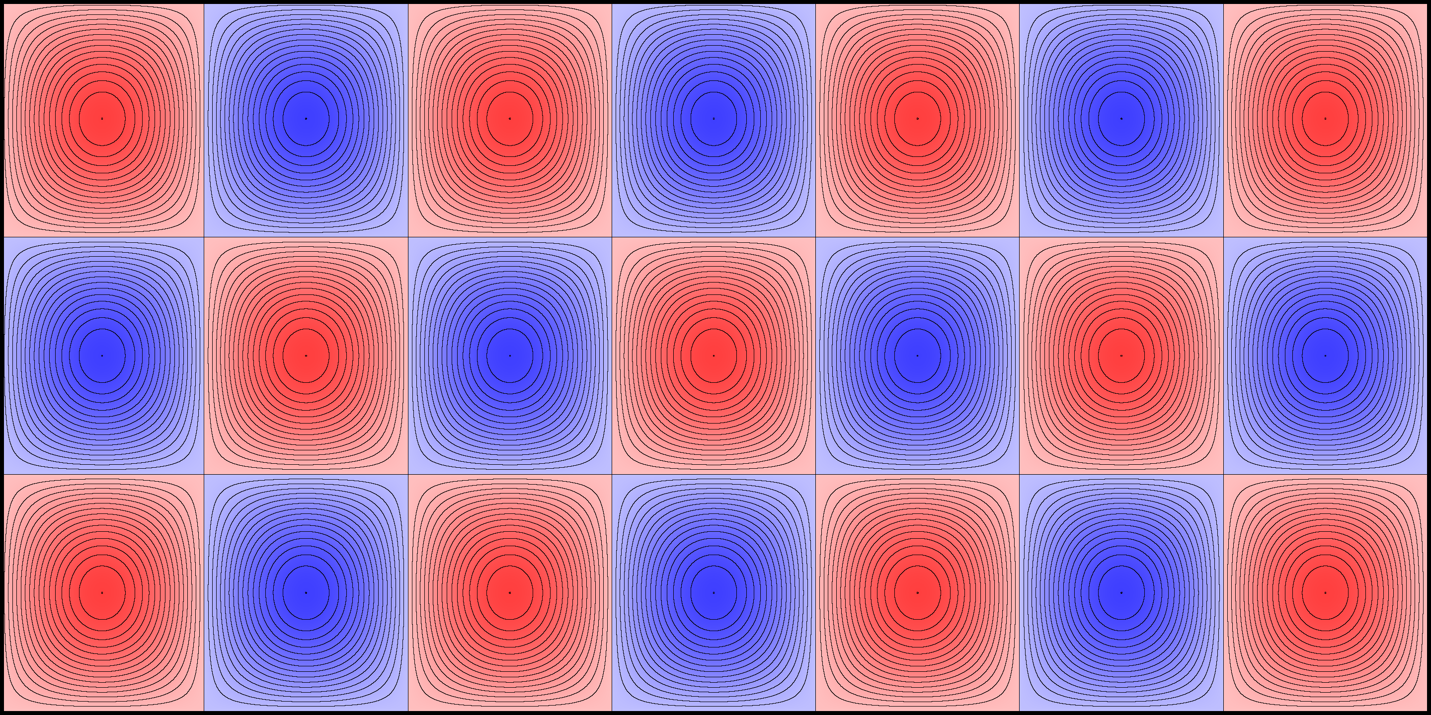
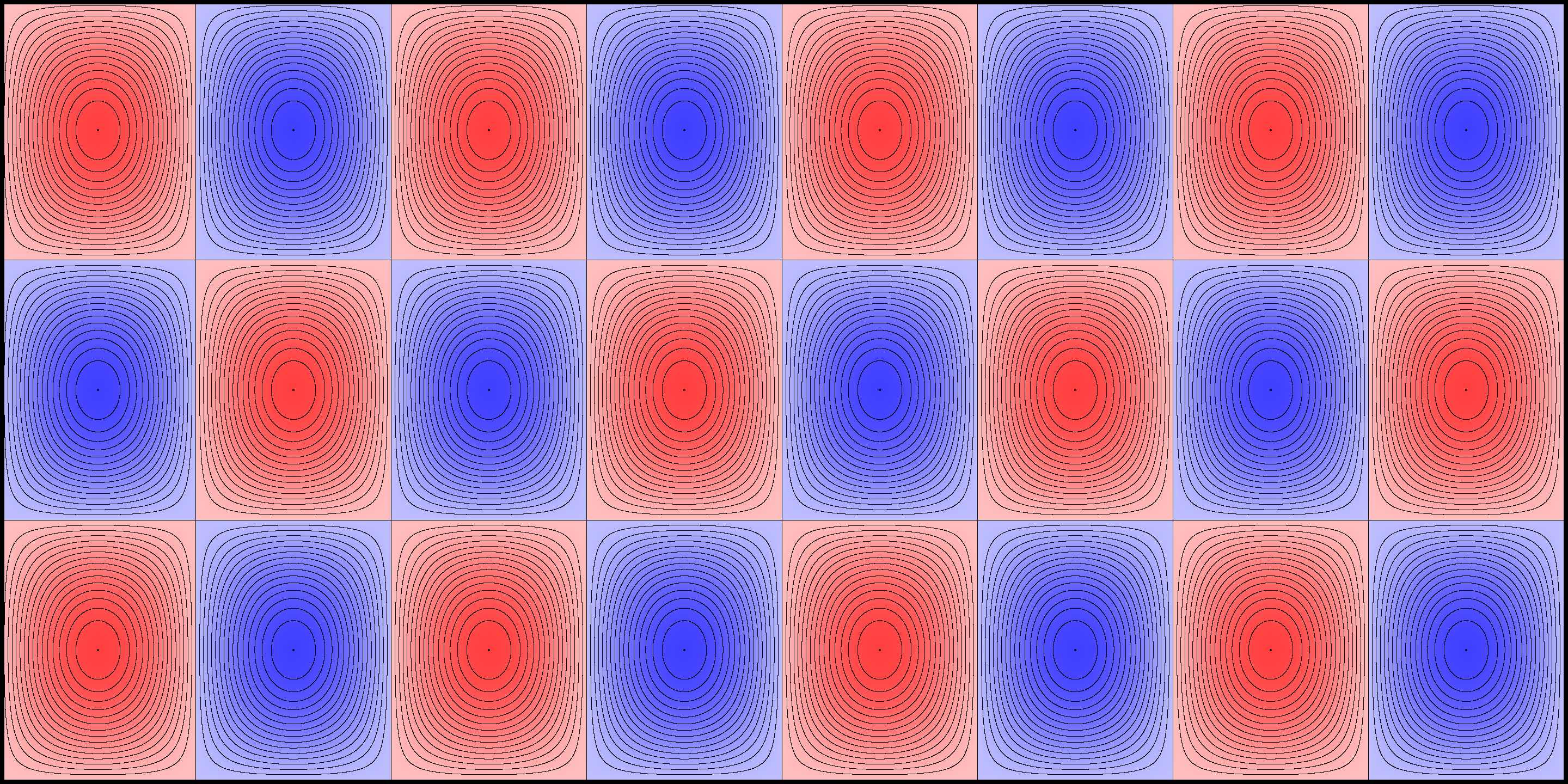
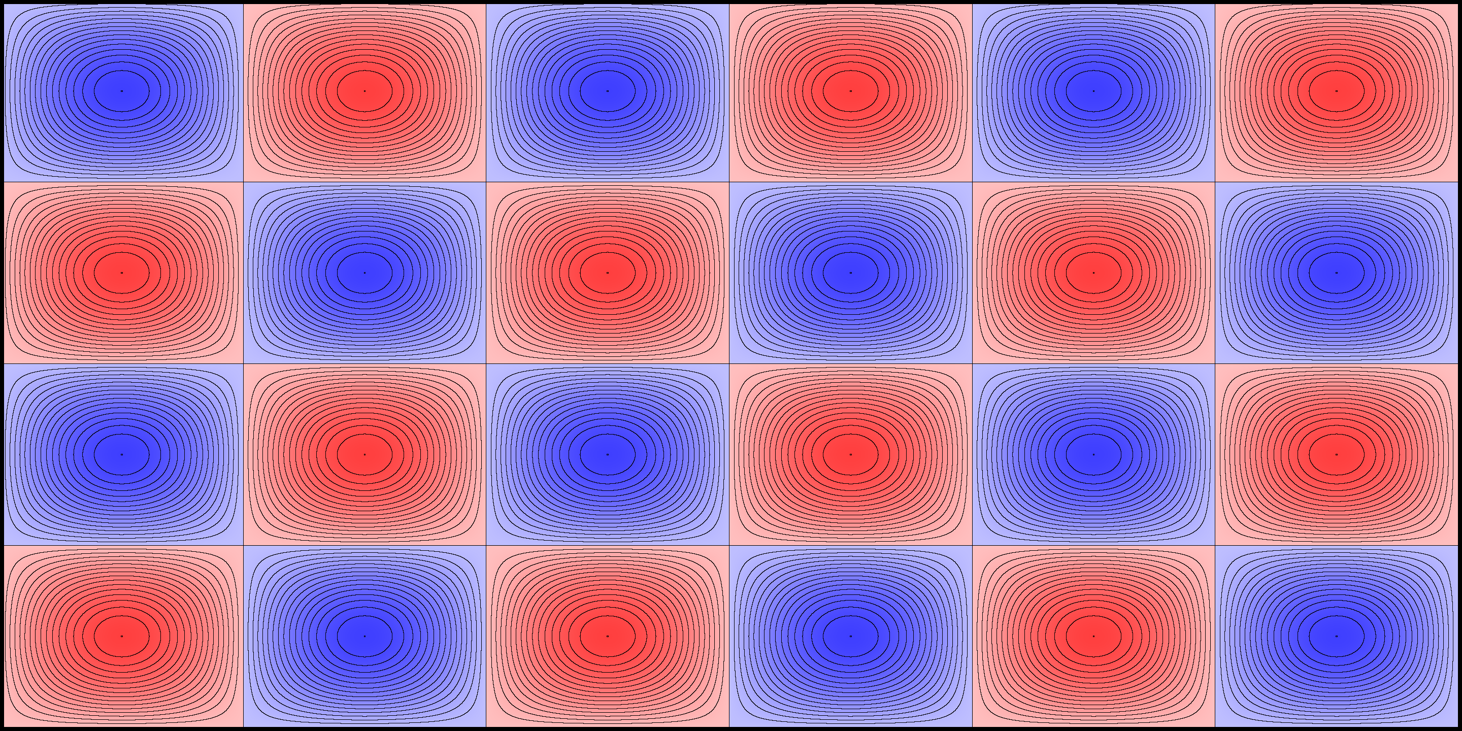
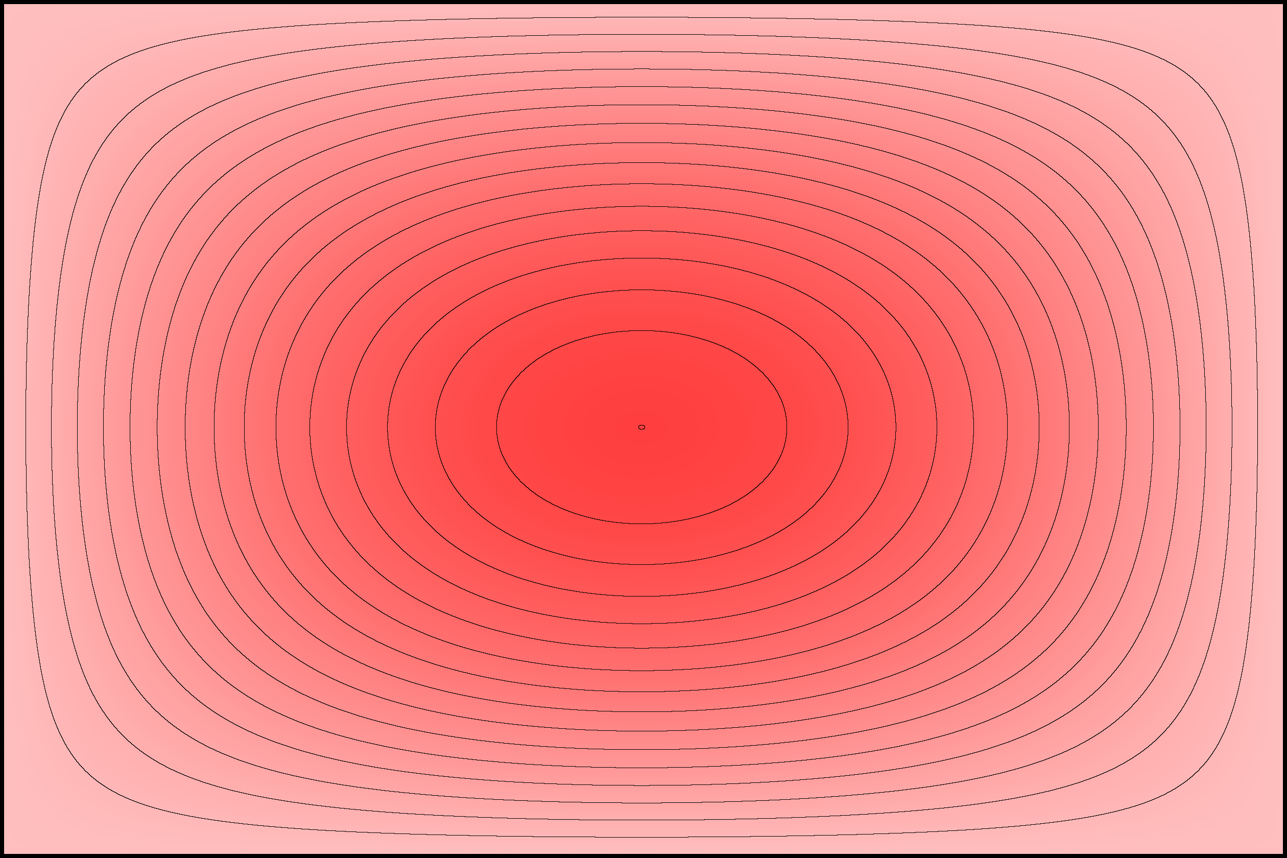
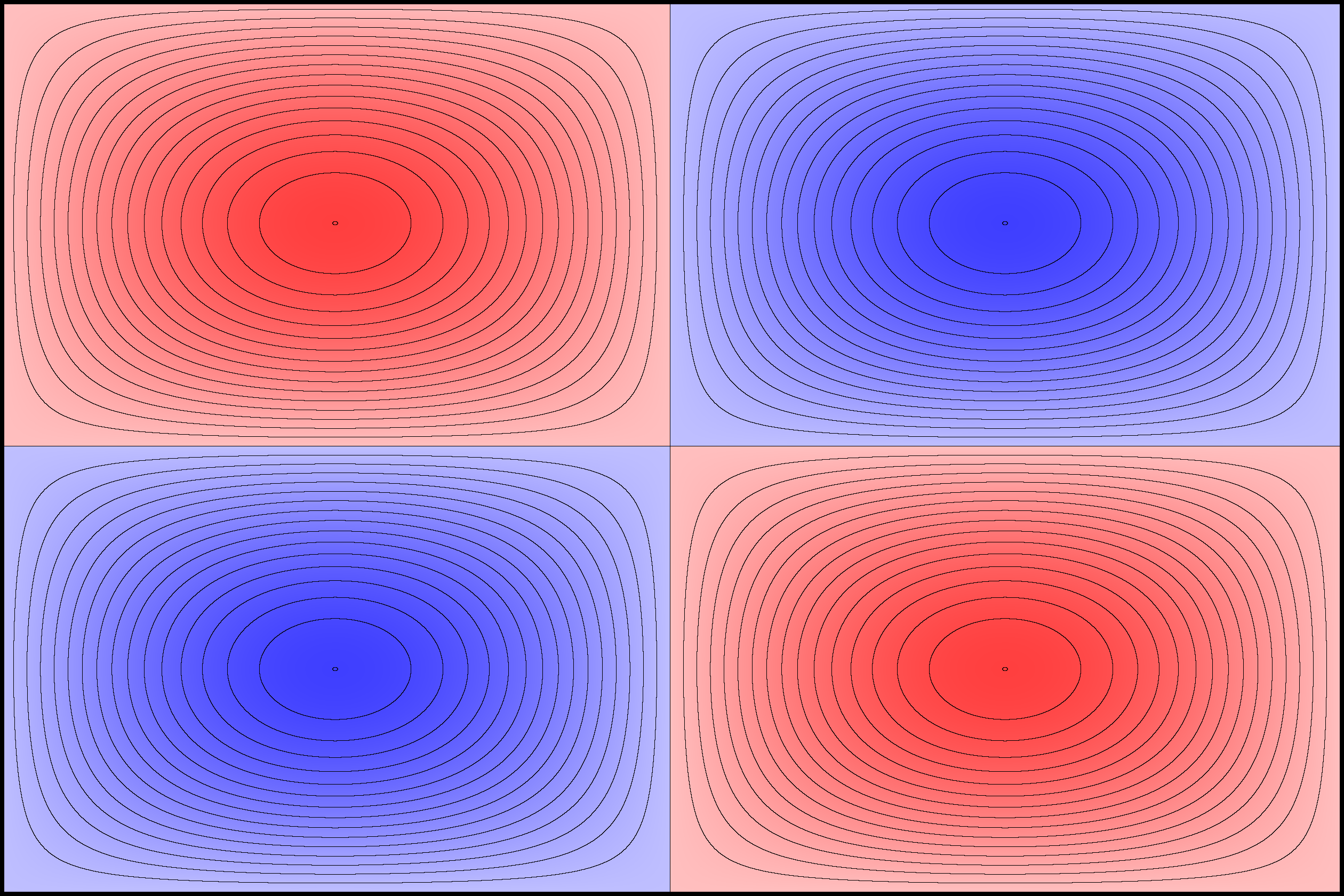
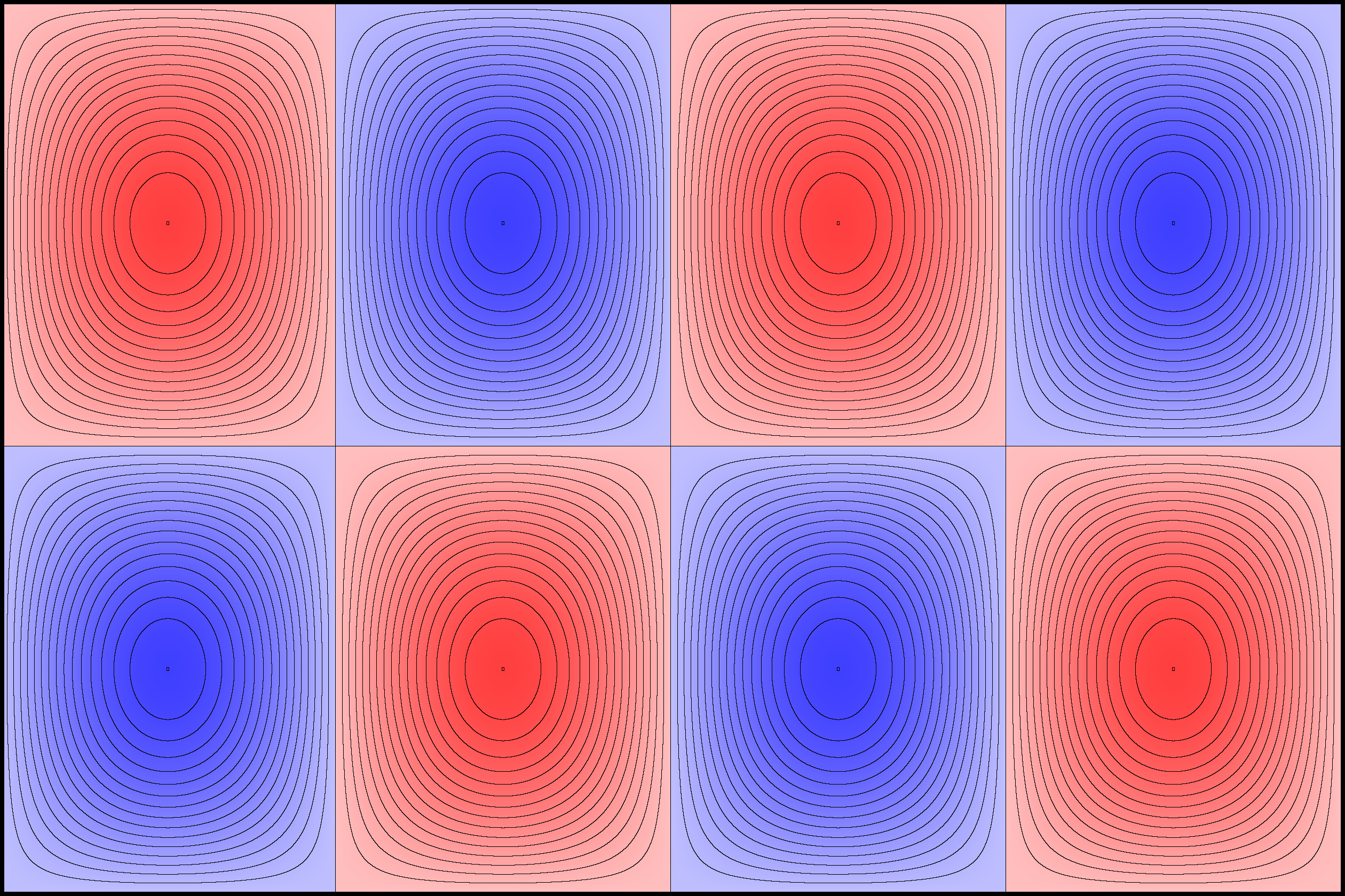
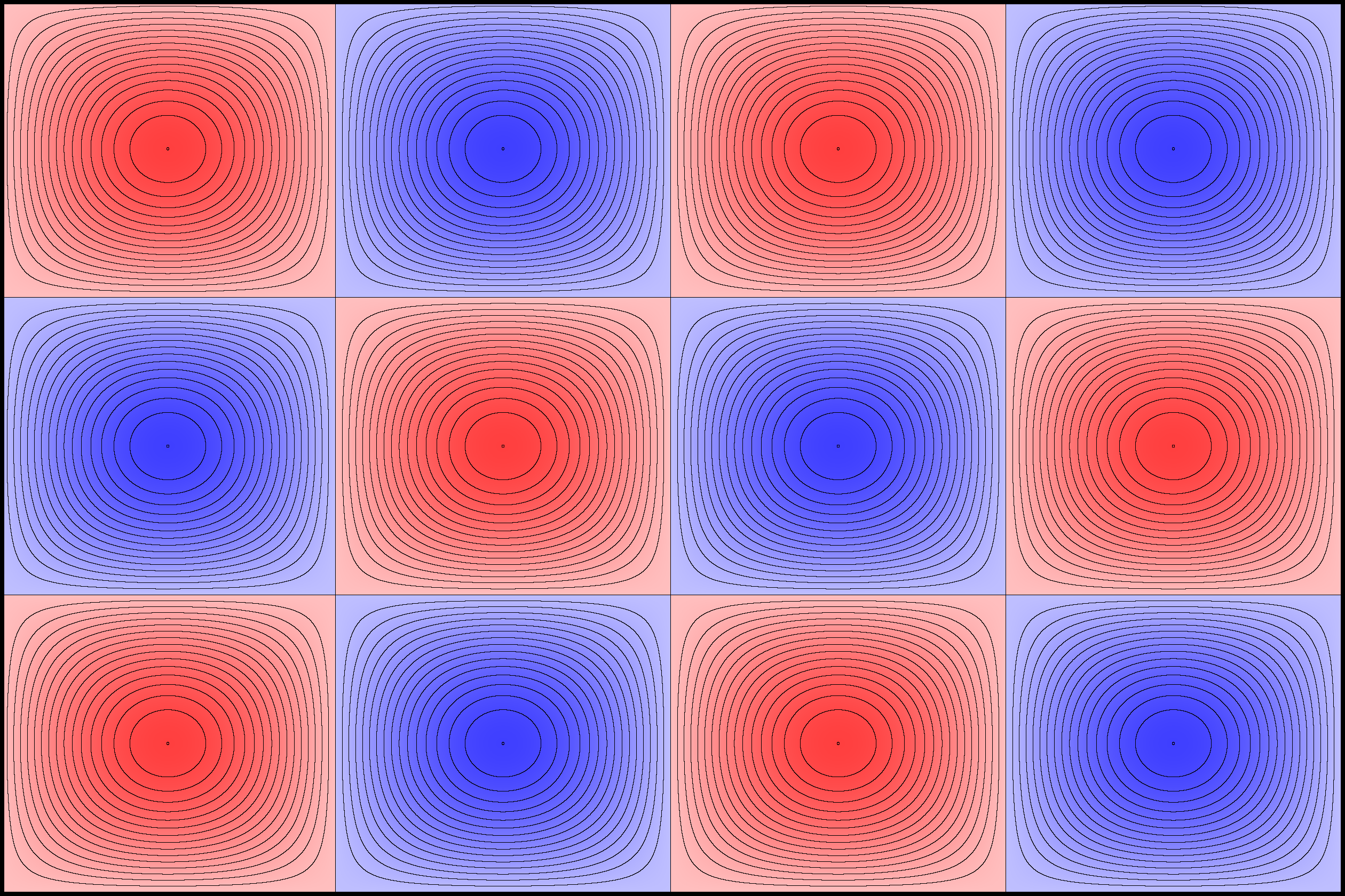
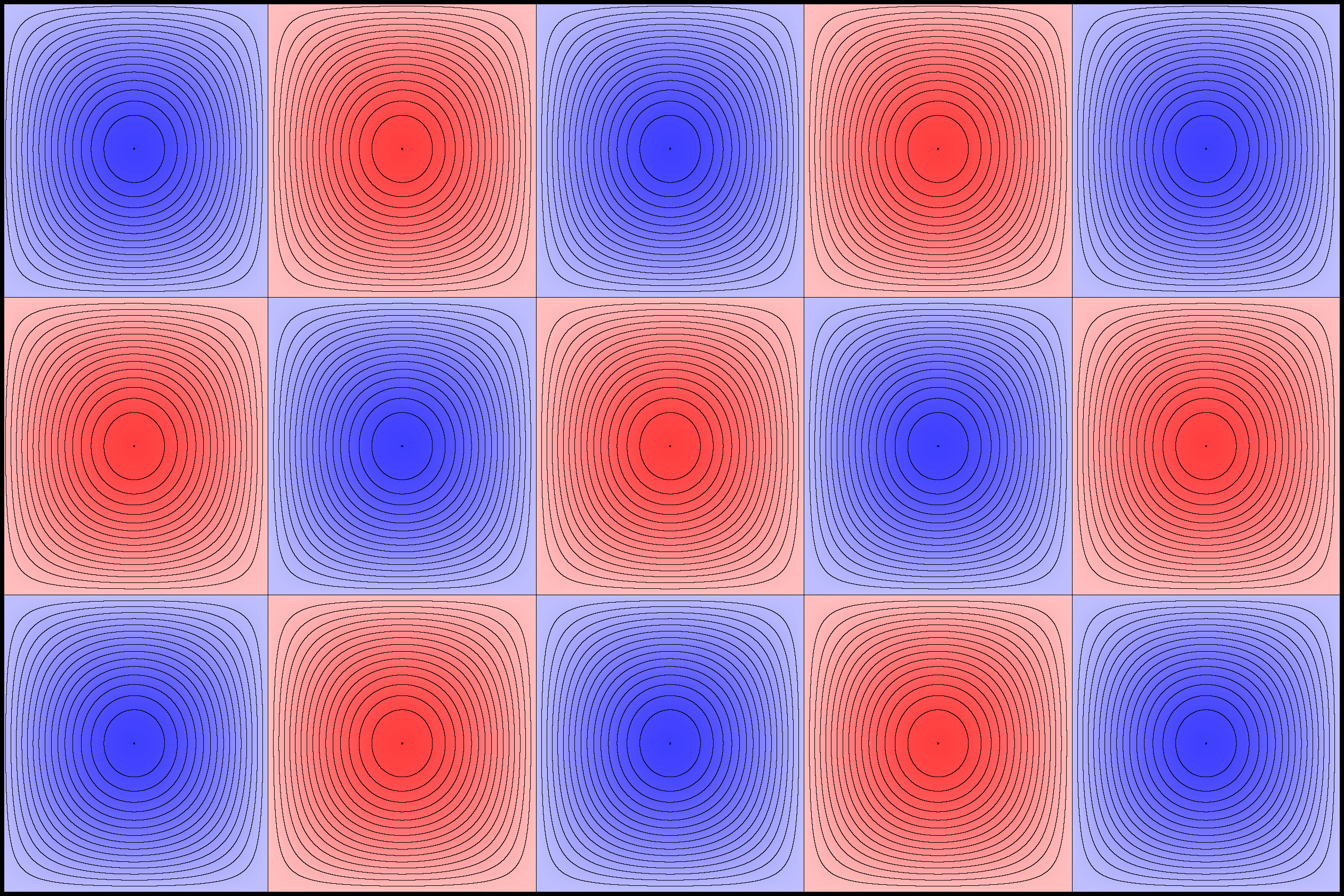
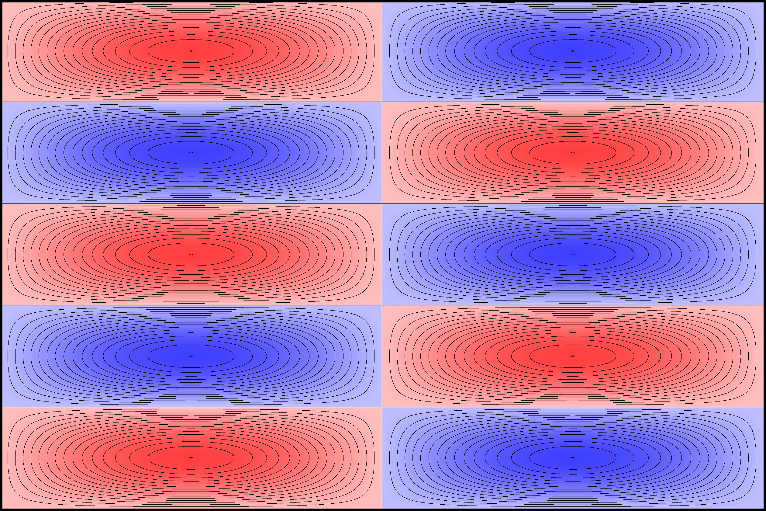
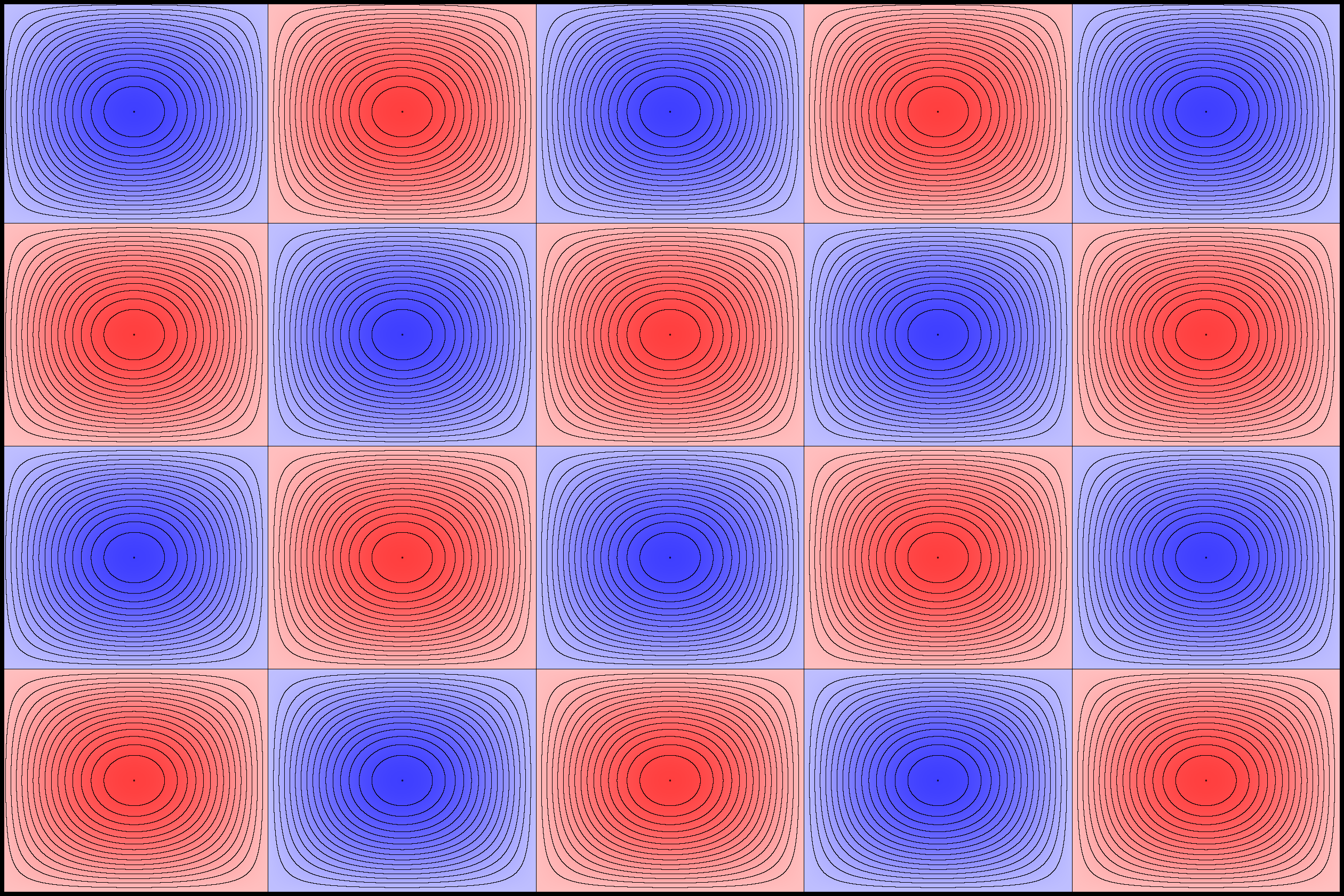
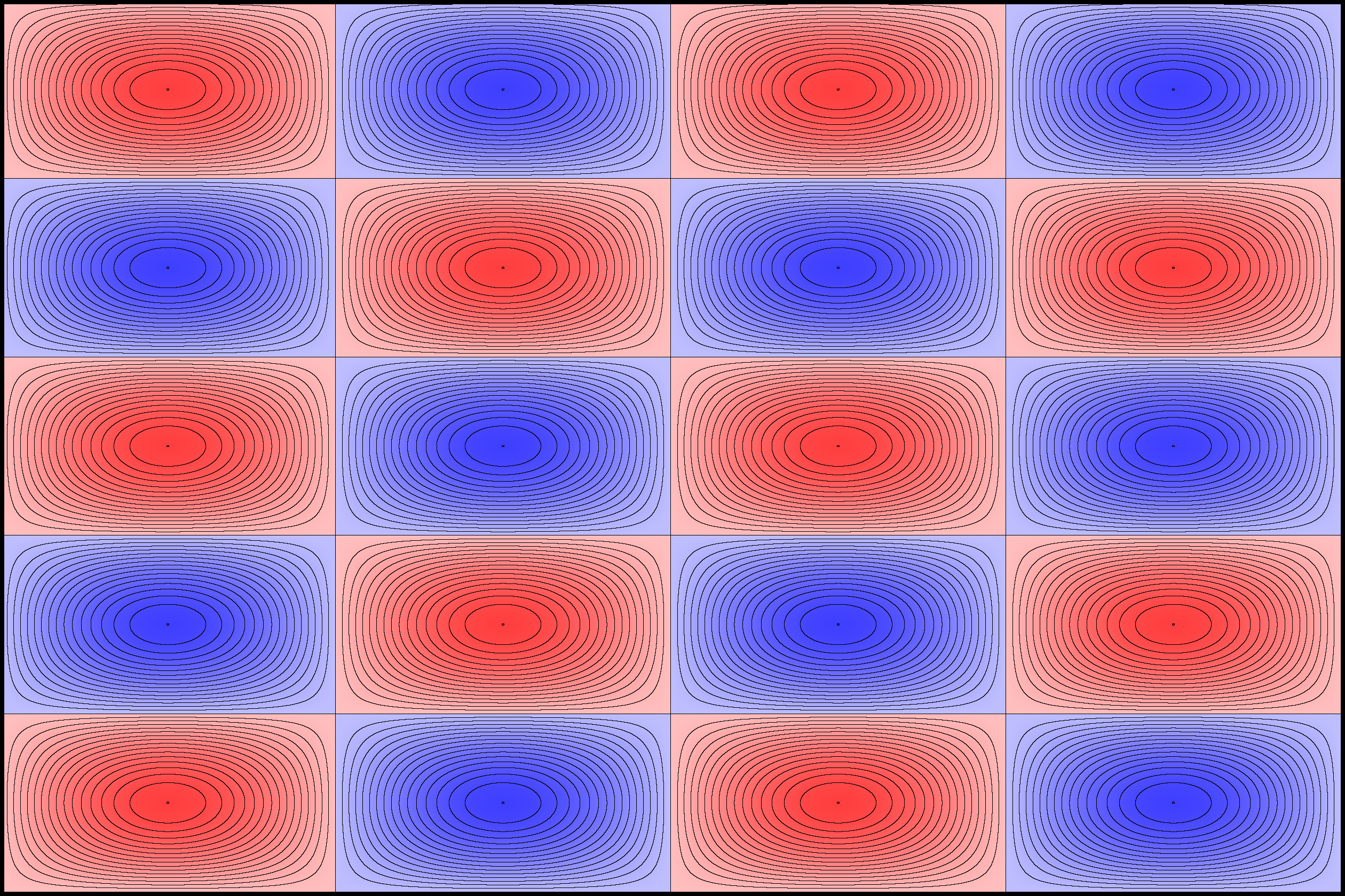
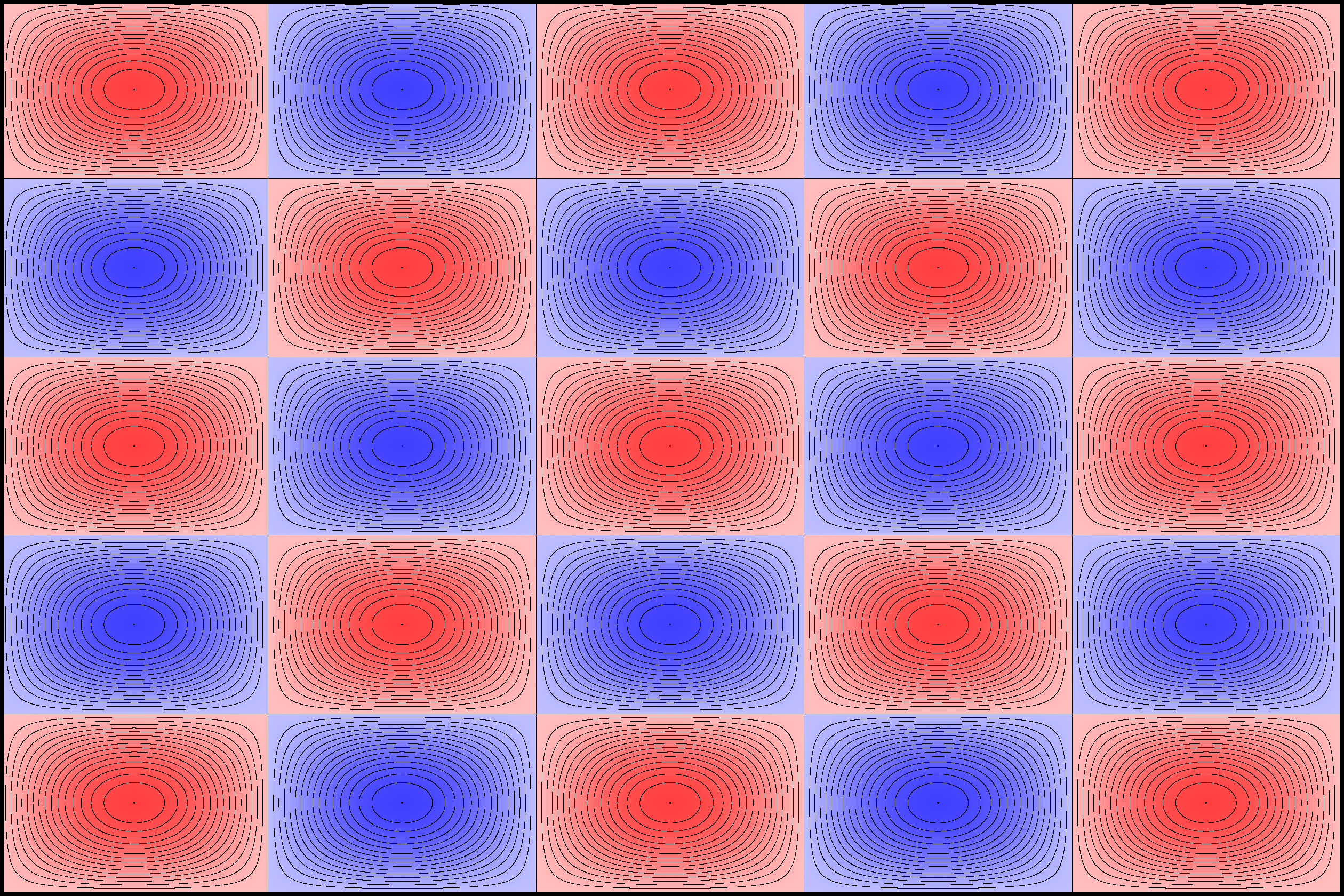
Experimenting with image manipulation in Octave was less fruitful, so I saved the raw data and processed it with a small C program. The grid sizes I used were around \(256 \times 256\). Constructing the sparse matrix took about 5 times longer than it took to solve the eigensystem, which goes to show that interpreted loops in Octave are to be avoided at all costs. Enough maths, here's some pictures, first some eigenmodes for square plate (I think some aren't as symmetric as they could be, due to duplicated eigenvalues giving a free choice of eigenvectors):

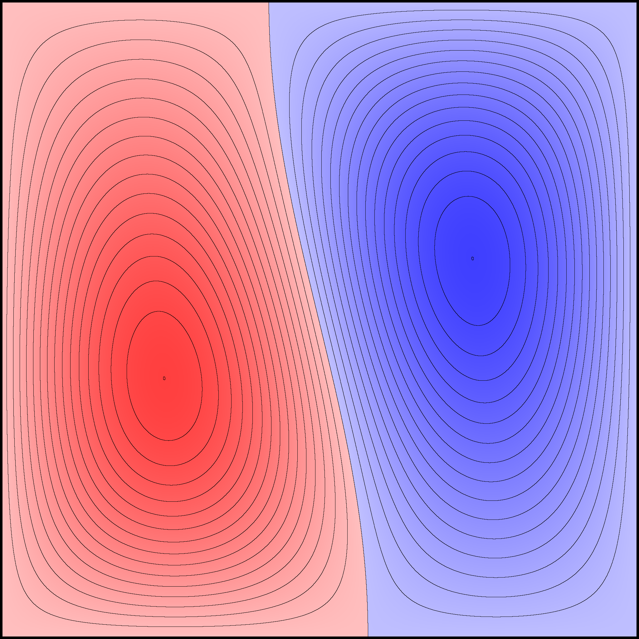
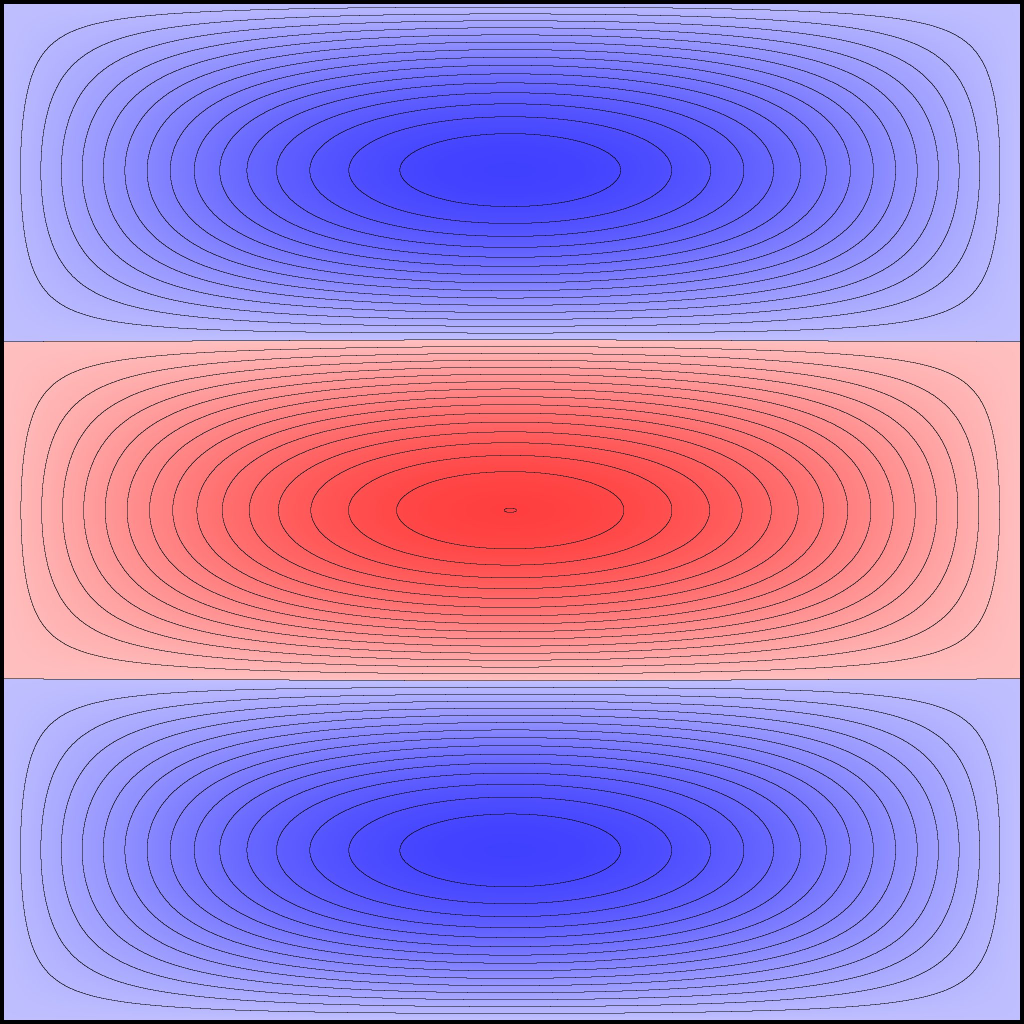
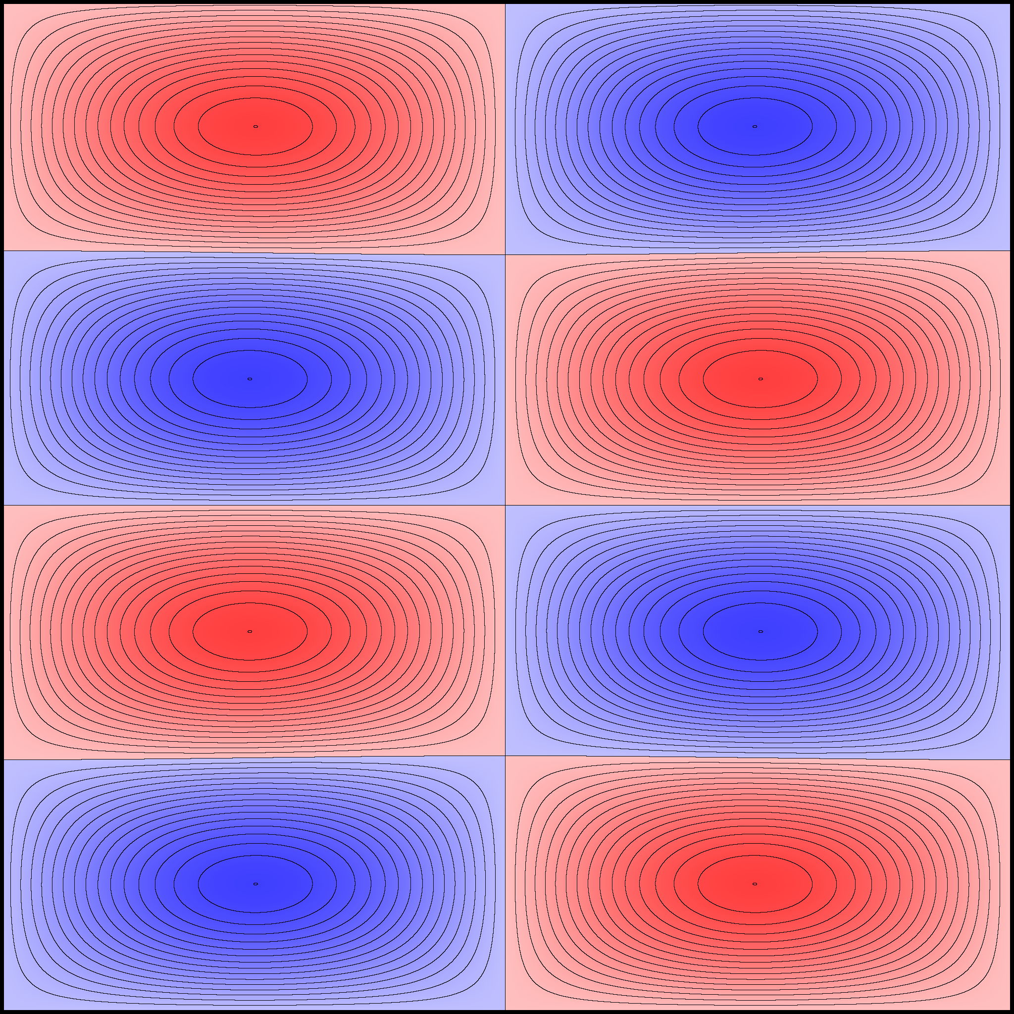
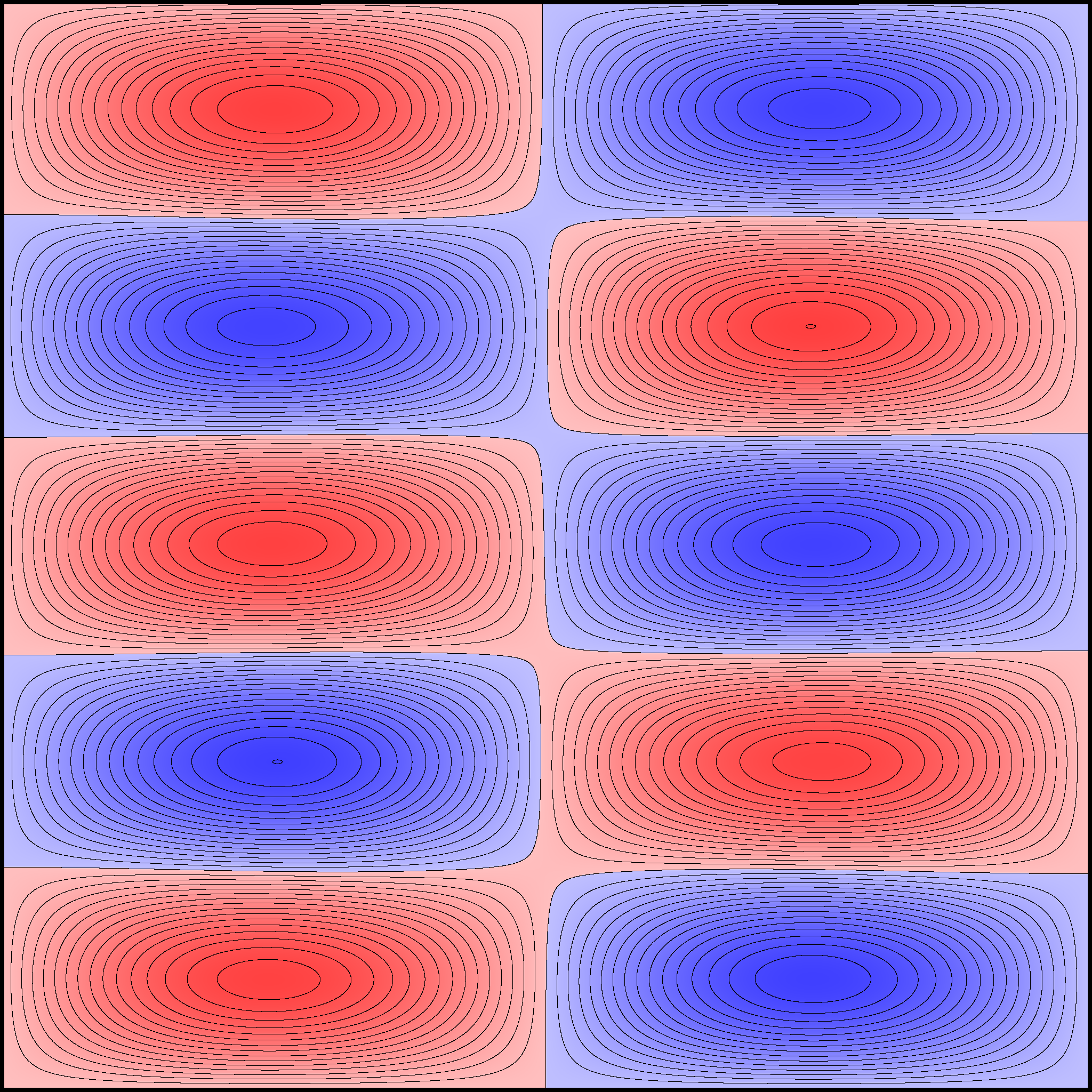
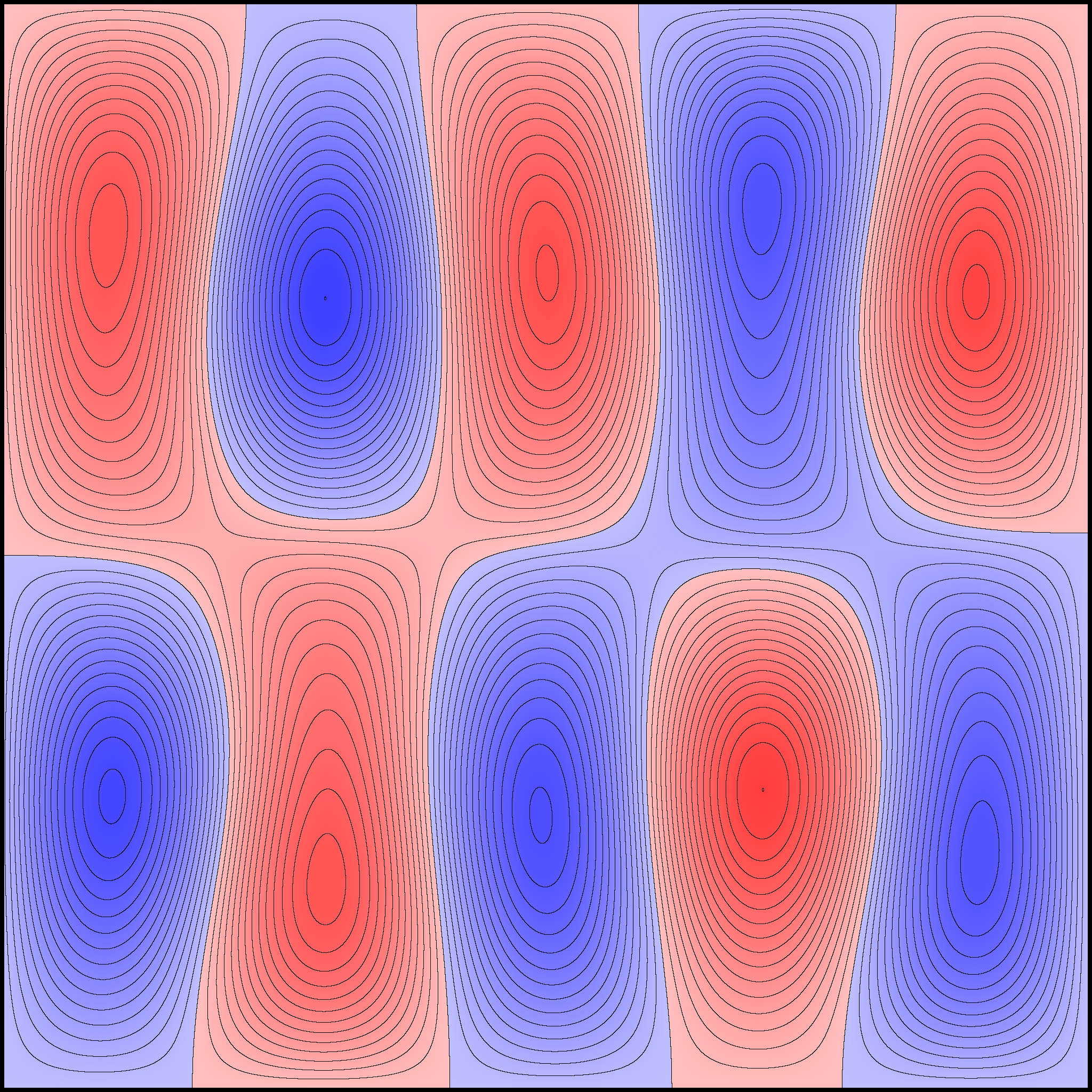
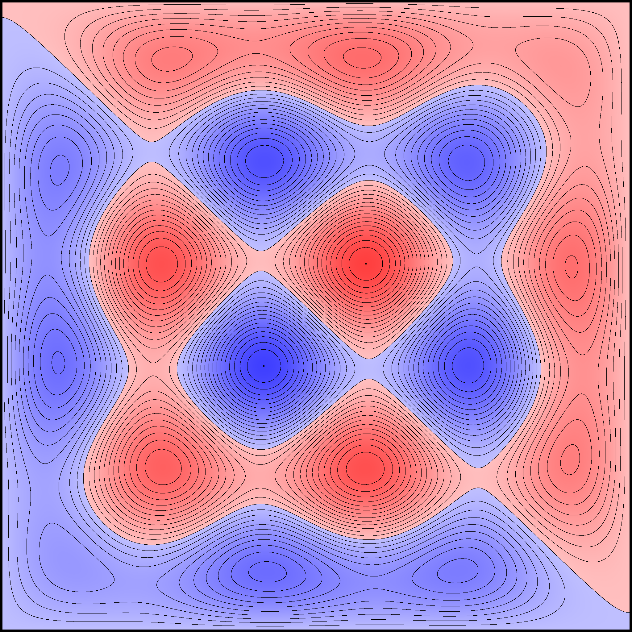
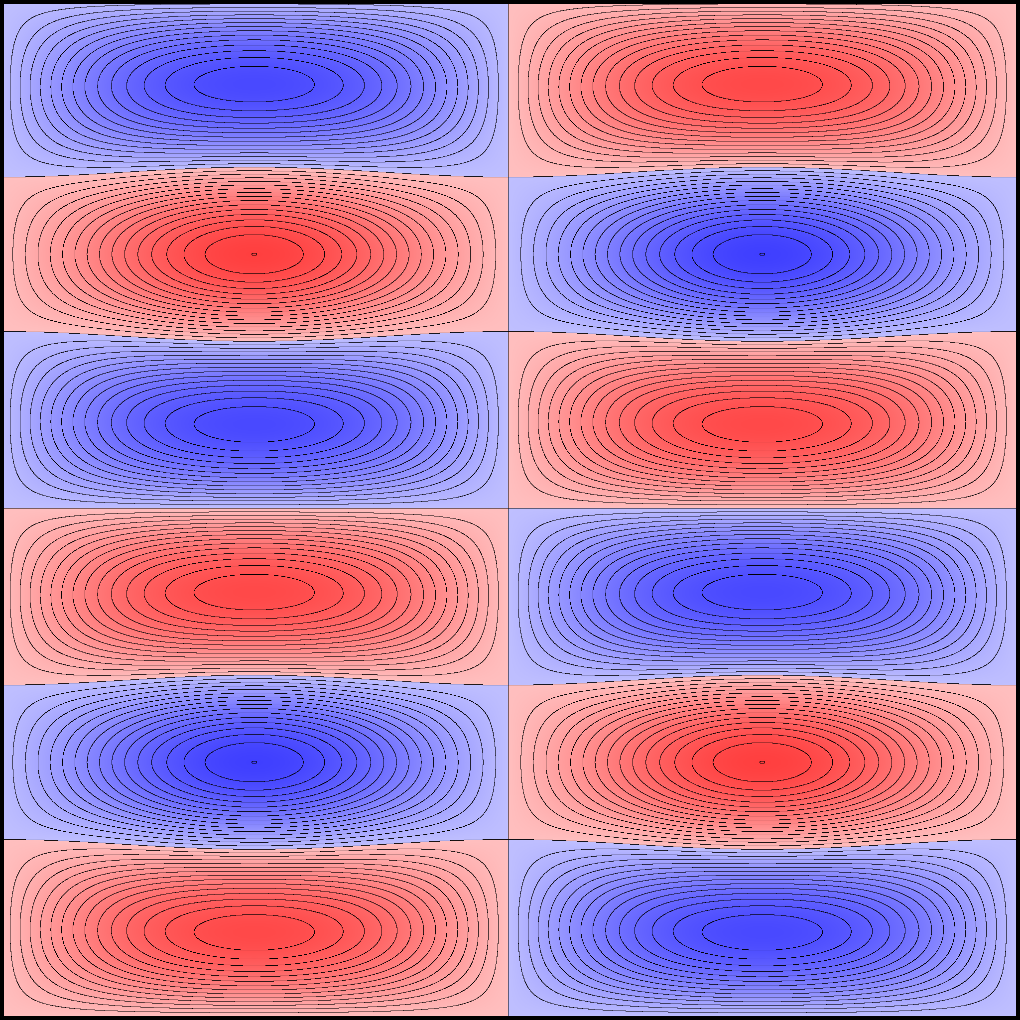
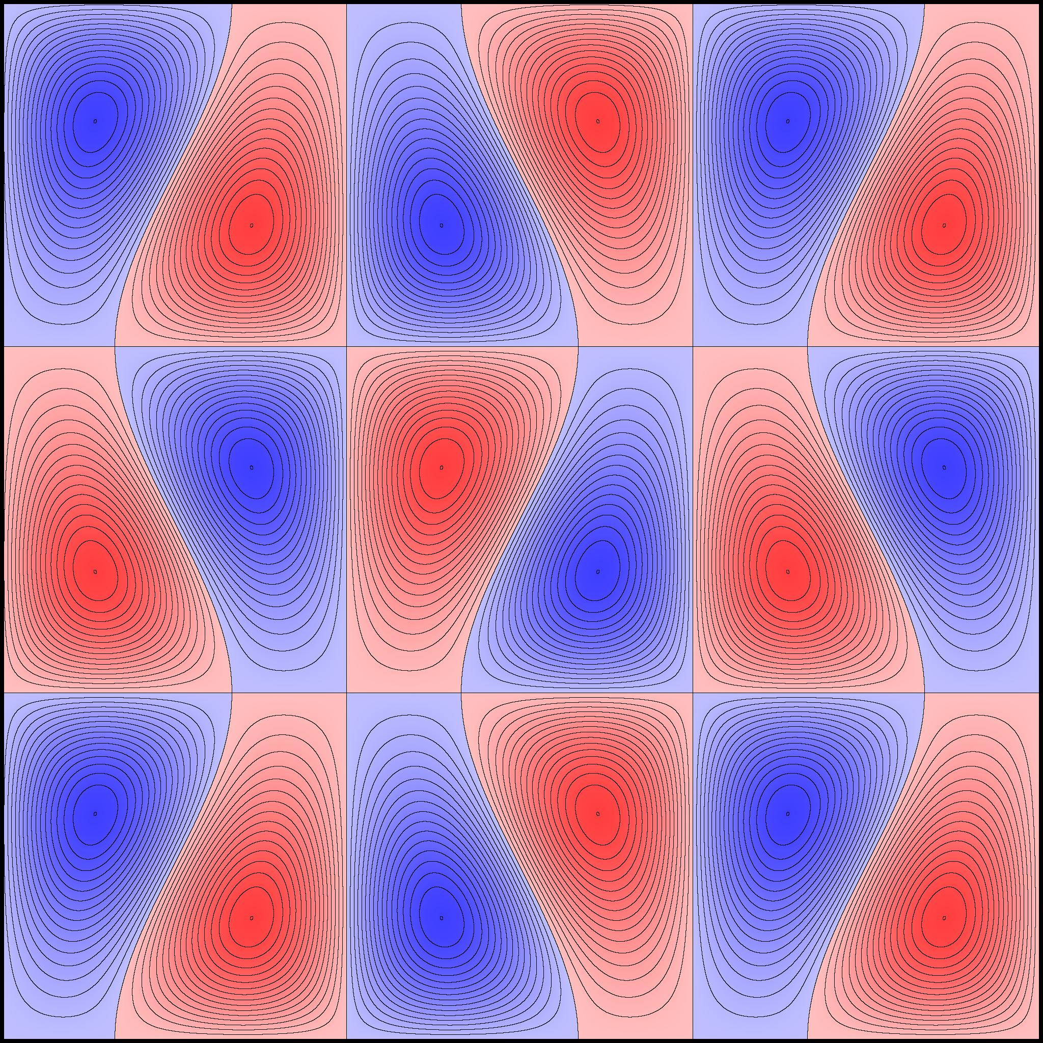
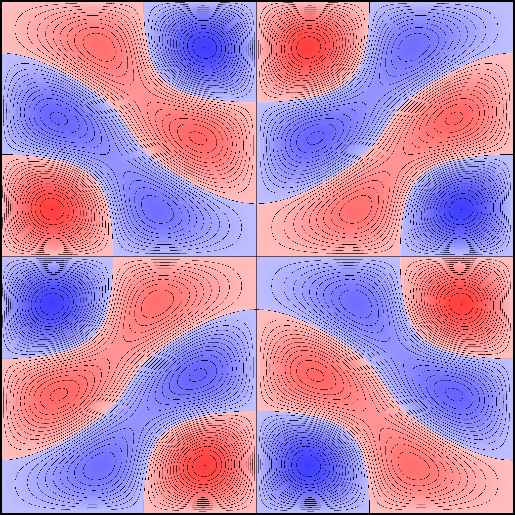
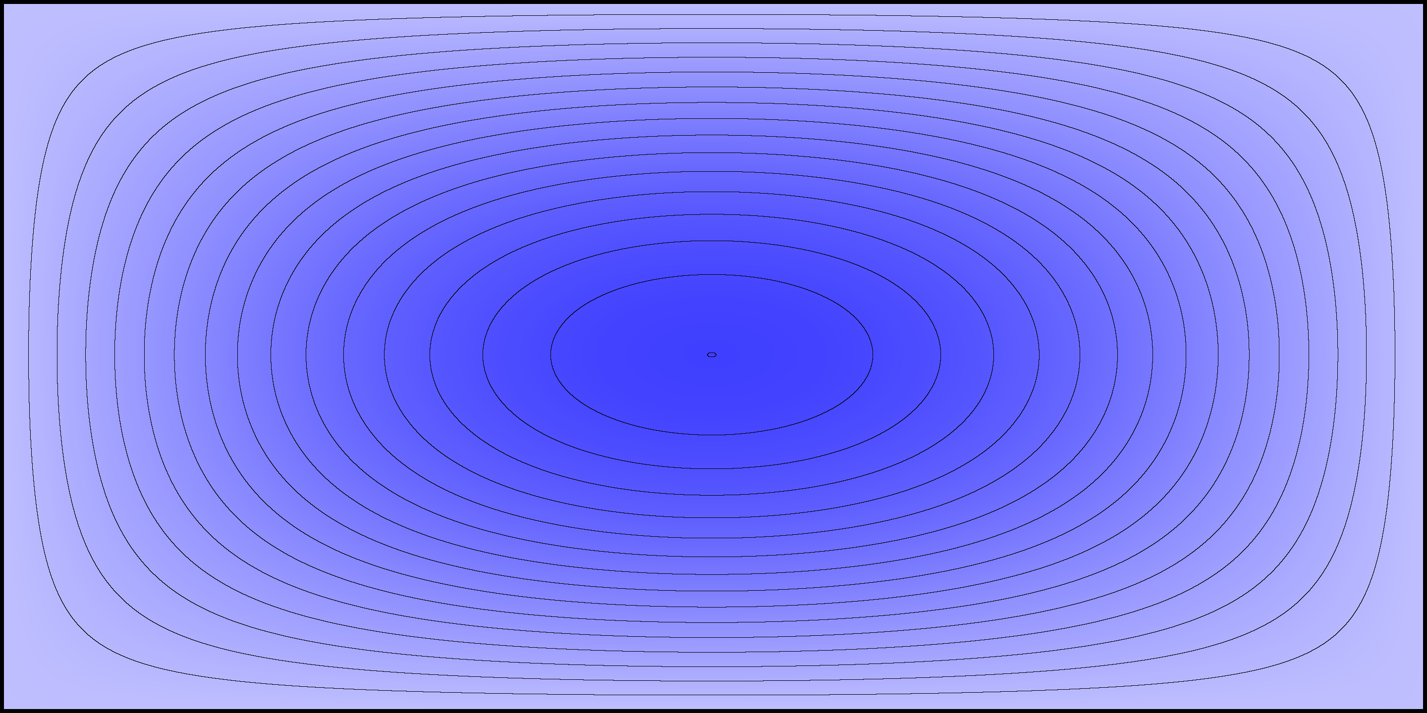
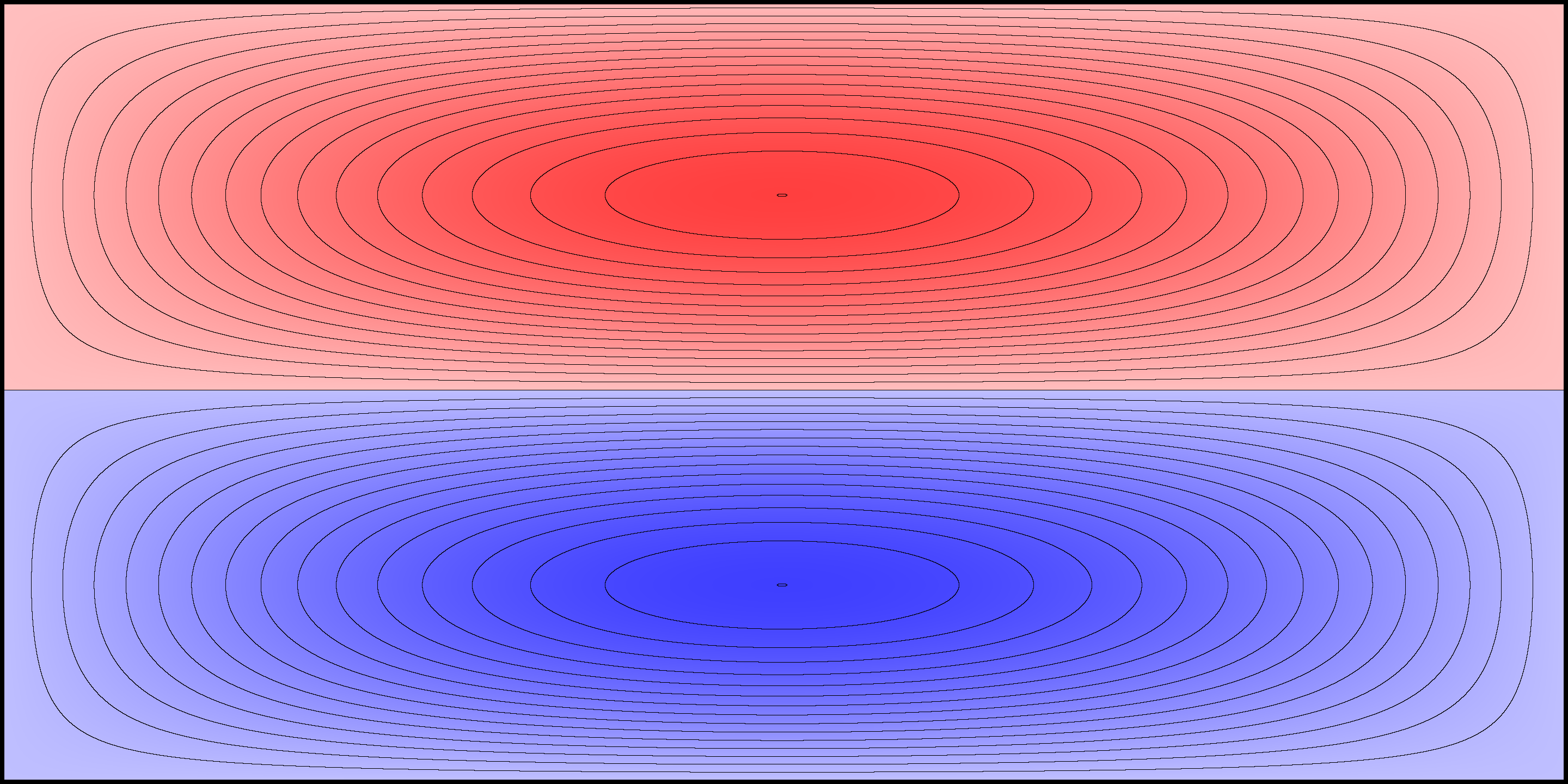
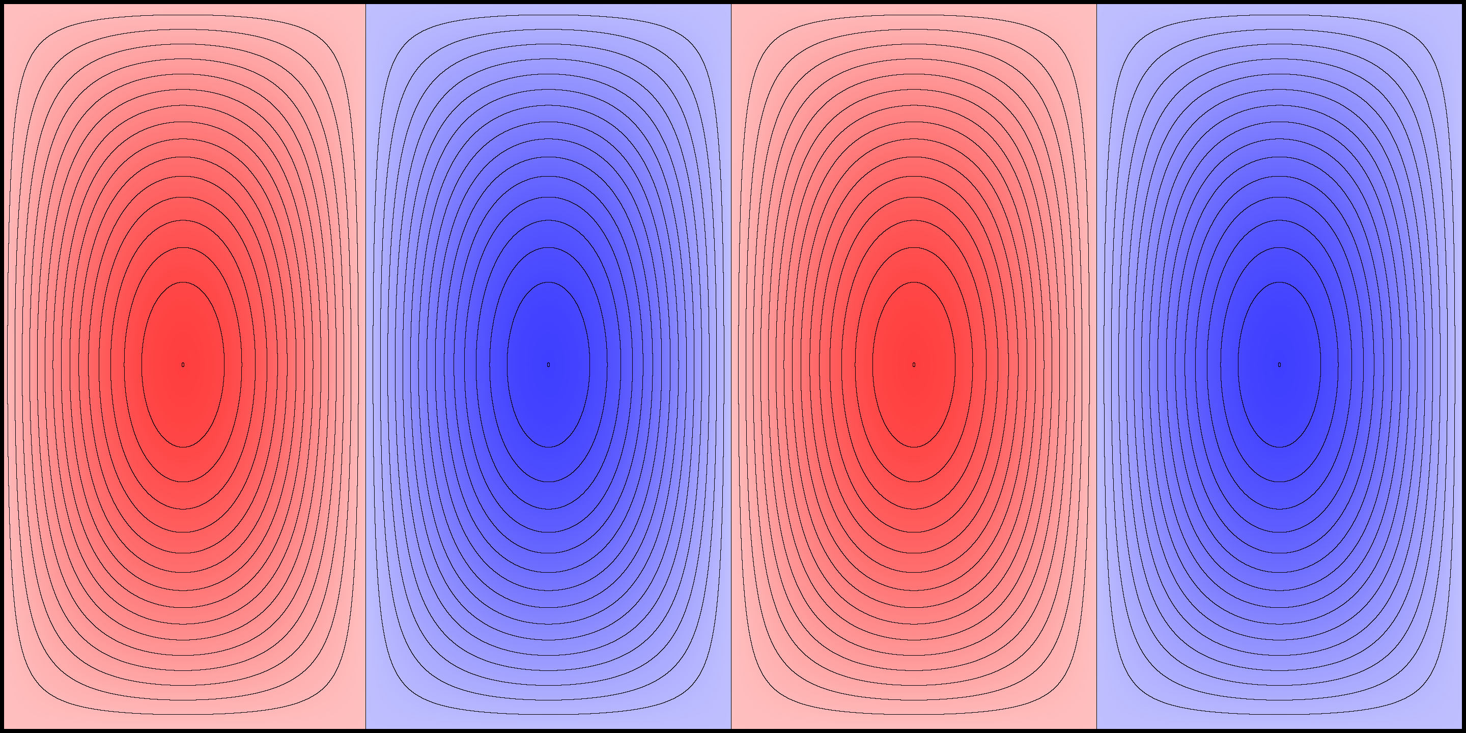
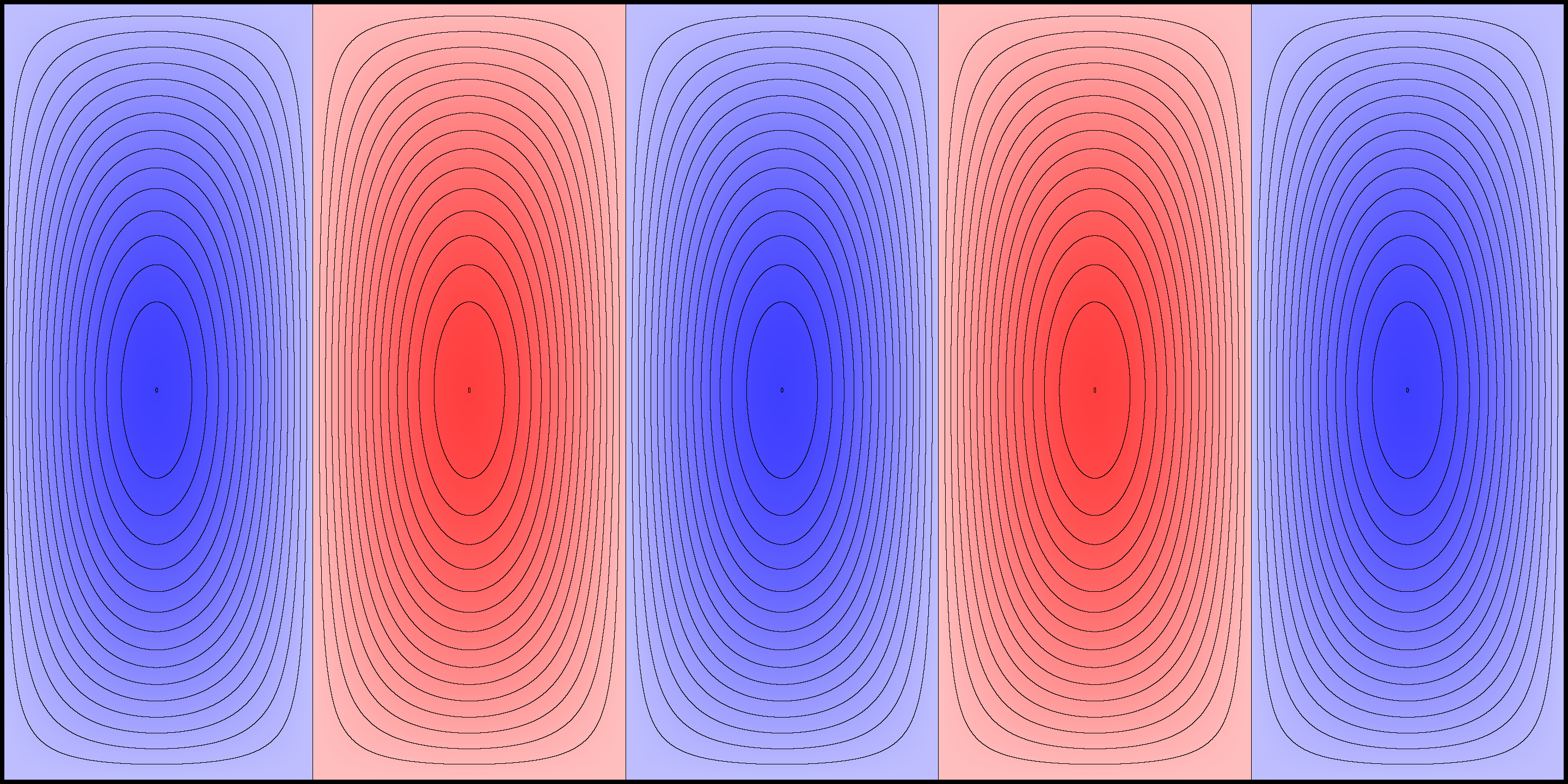
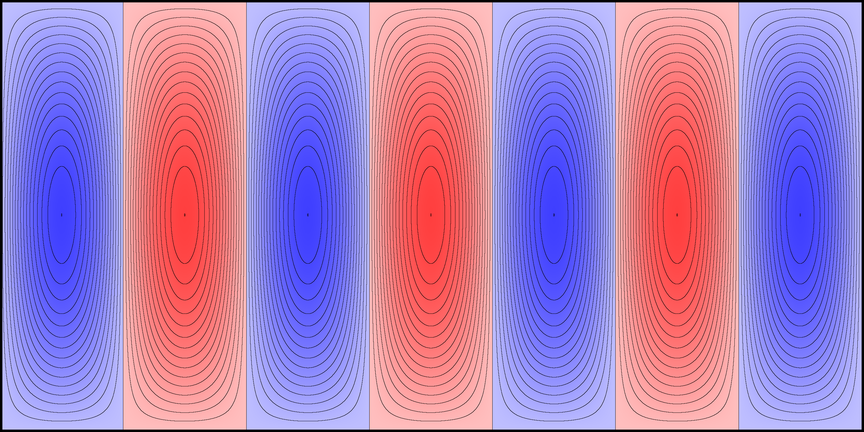
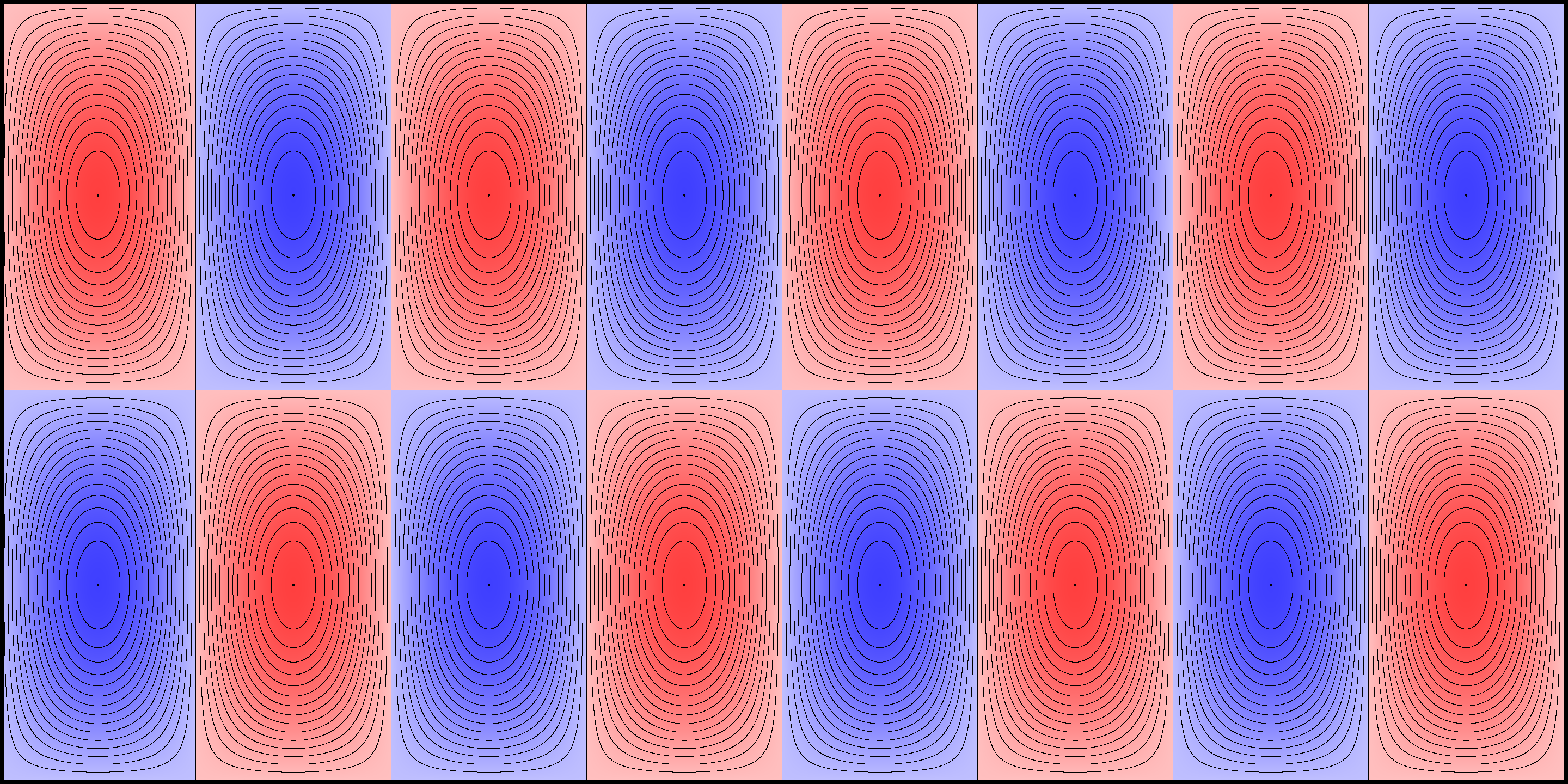
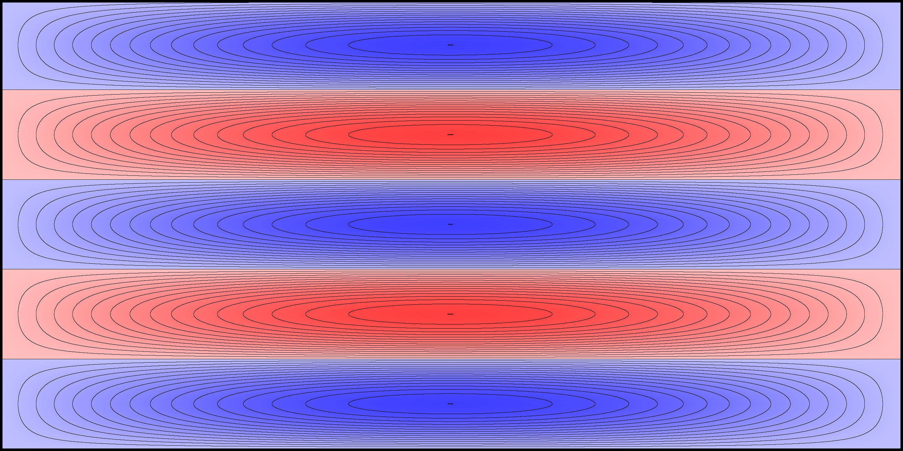
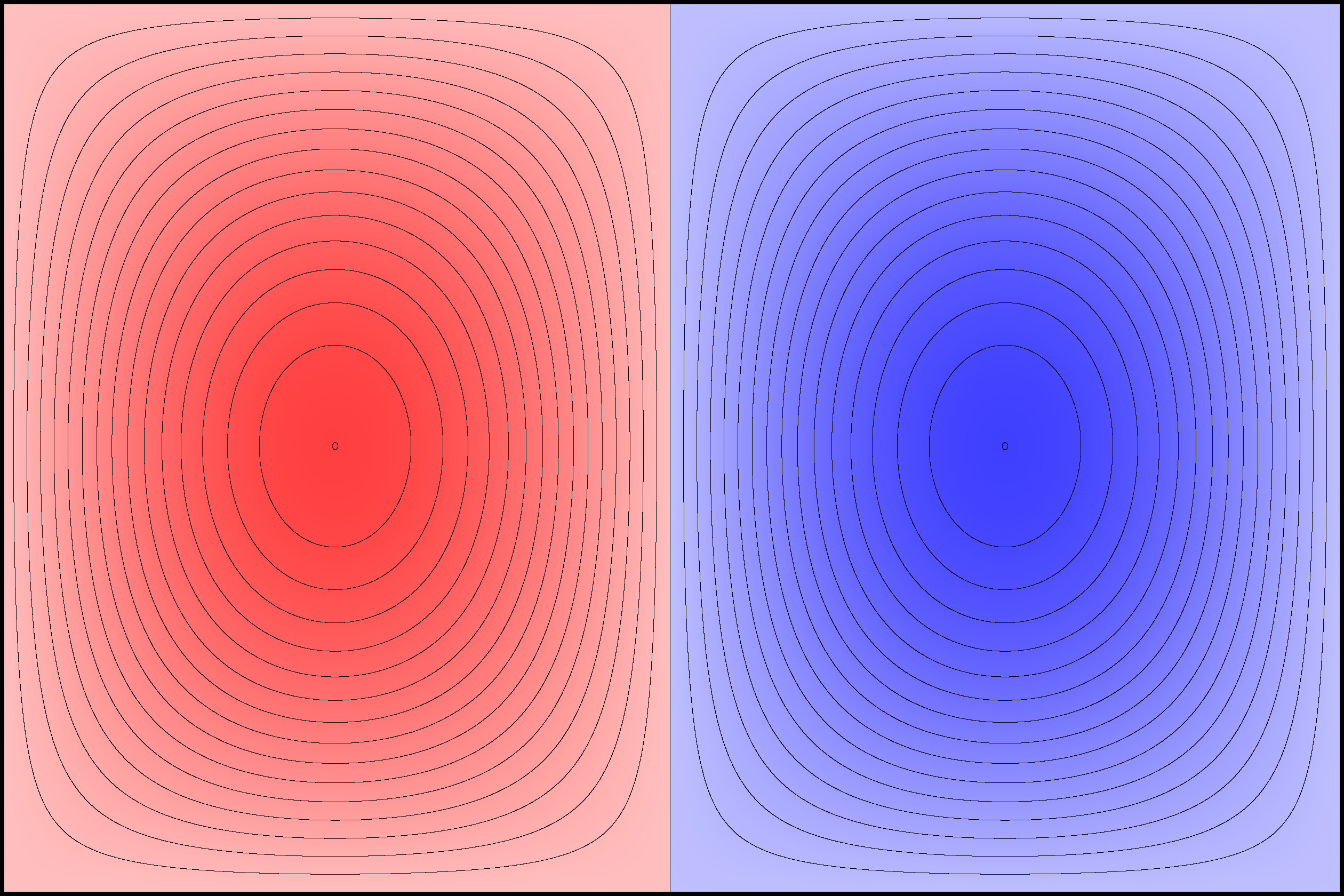
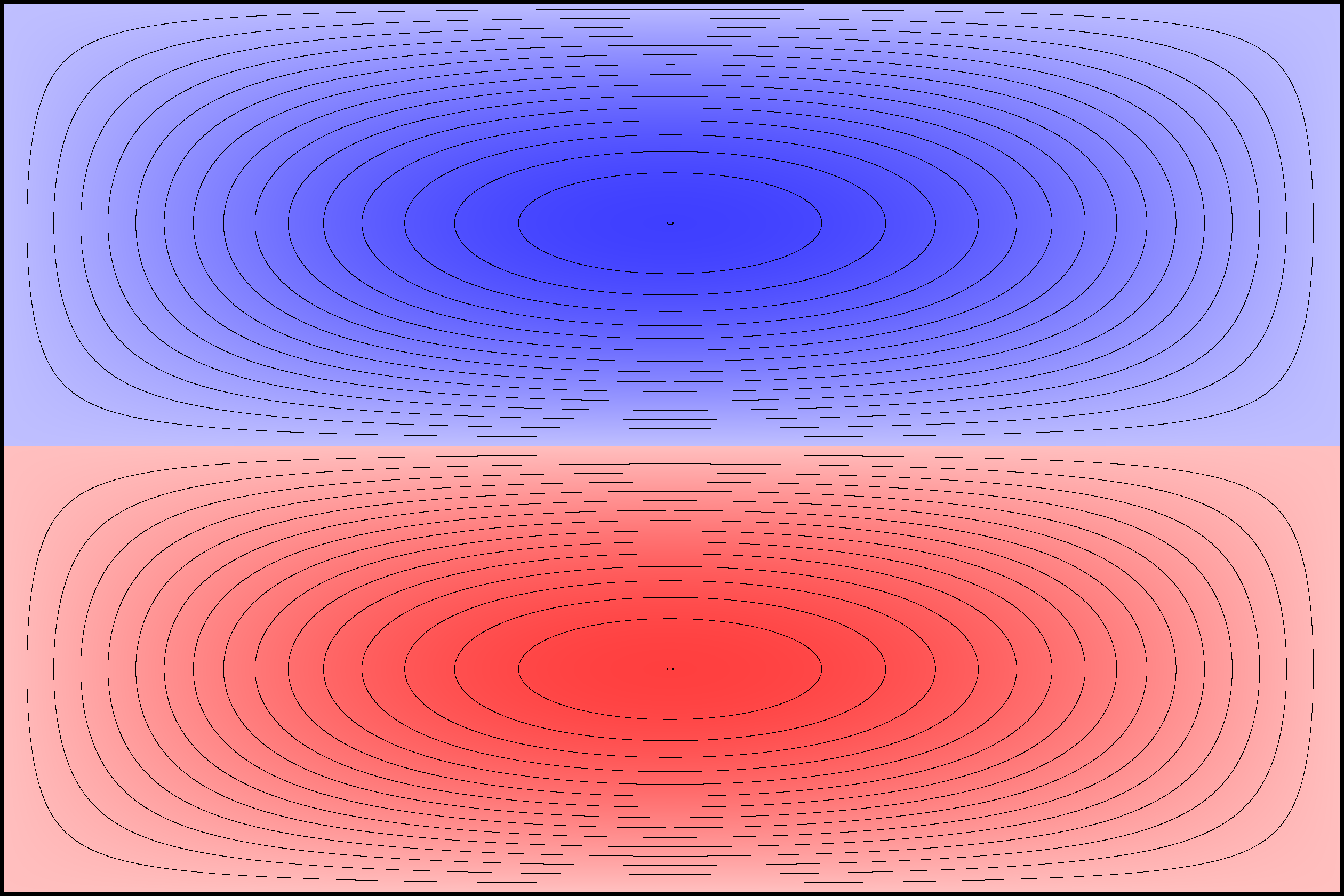
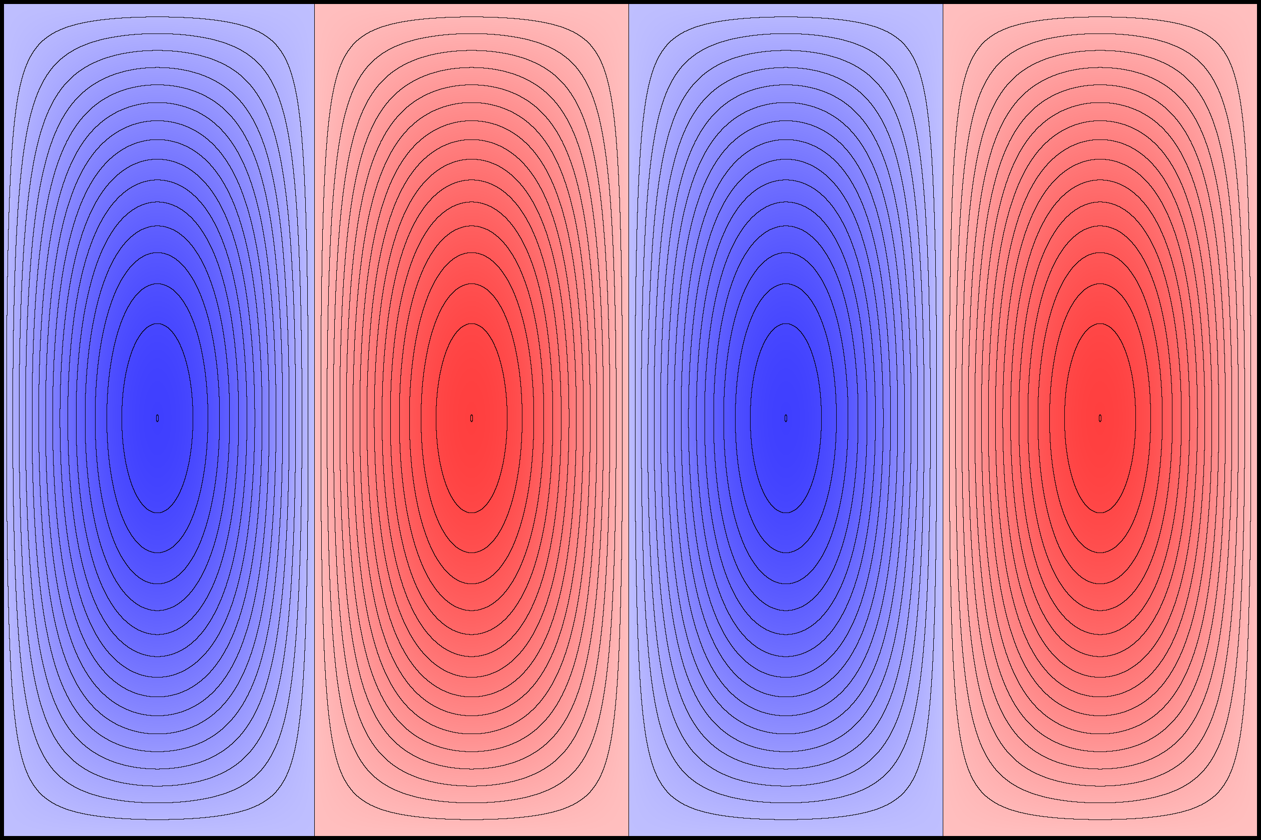
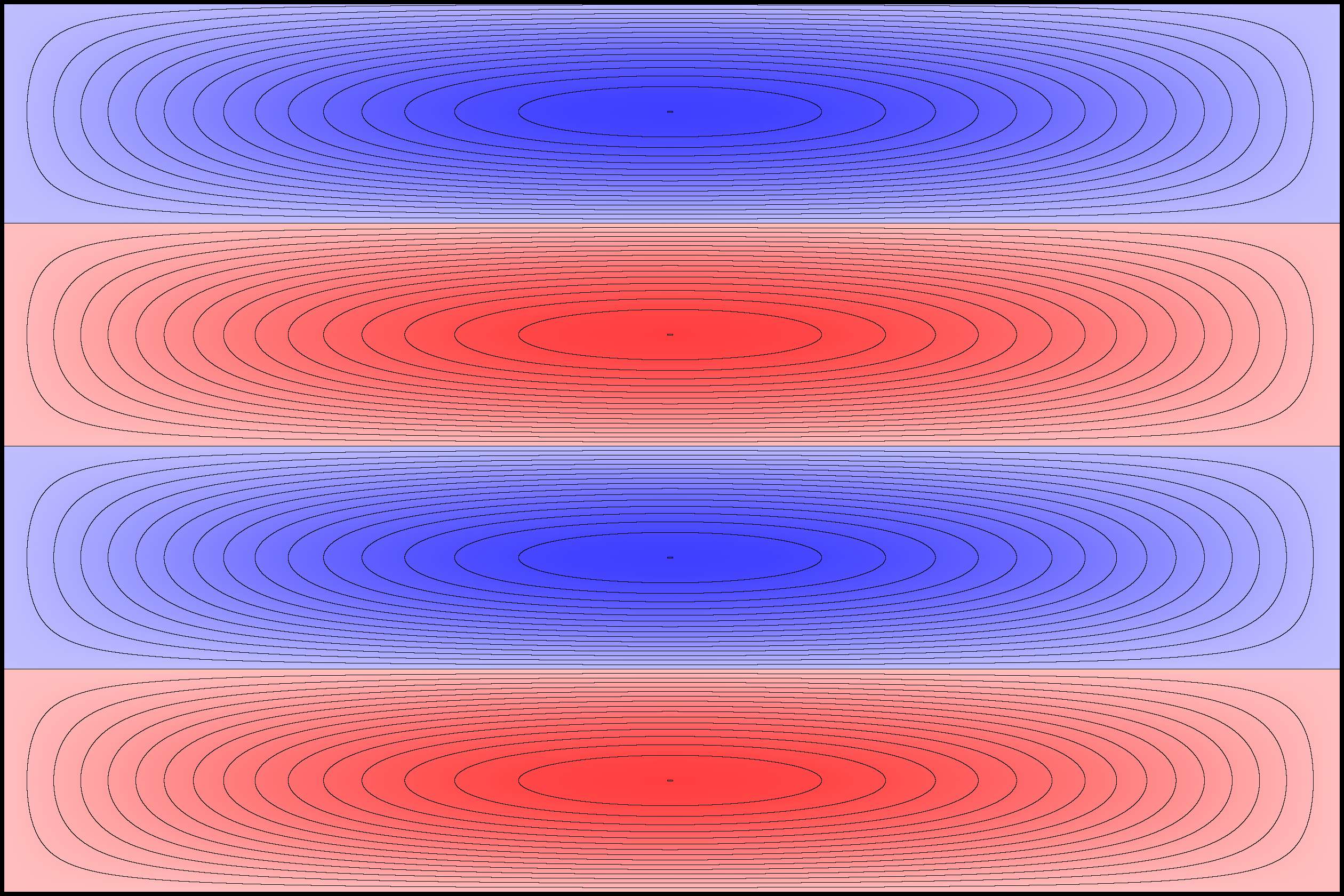
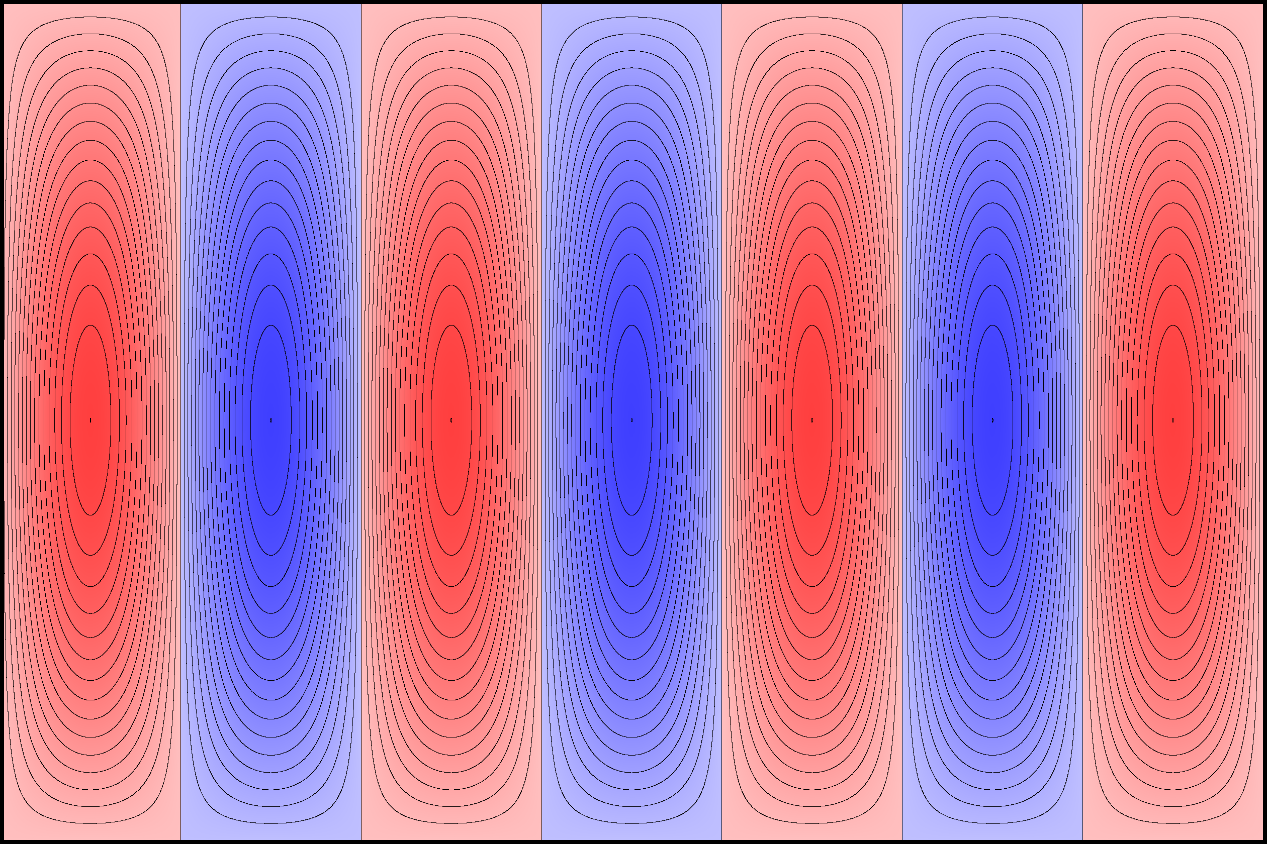
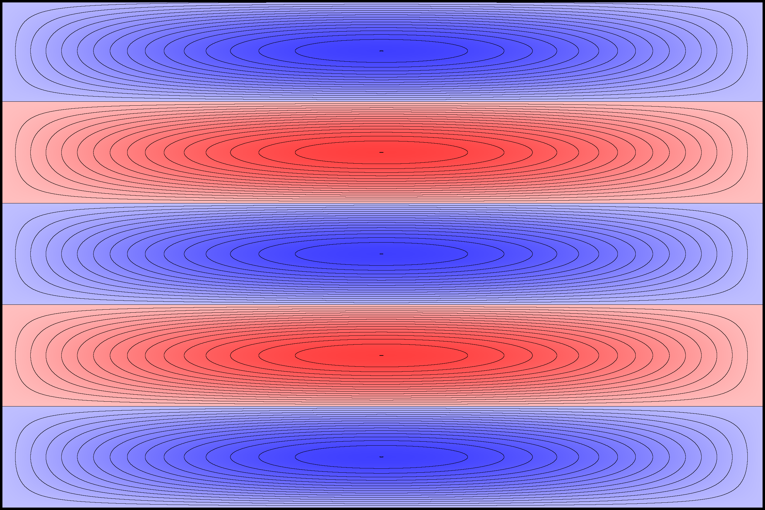
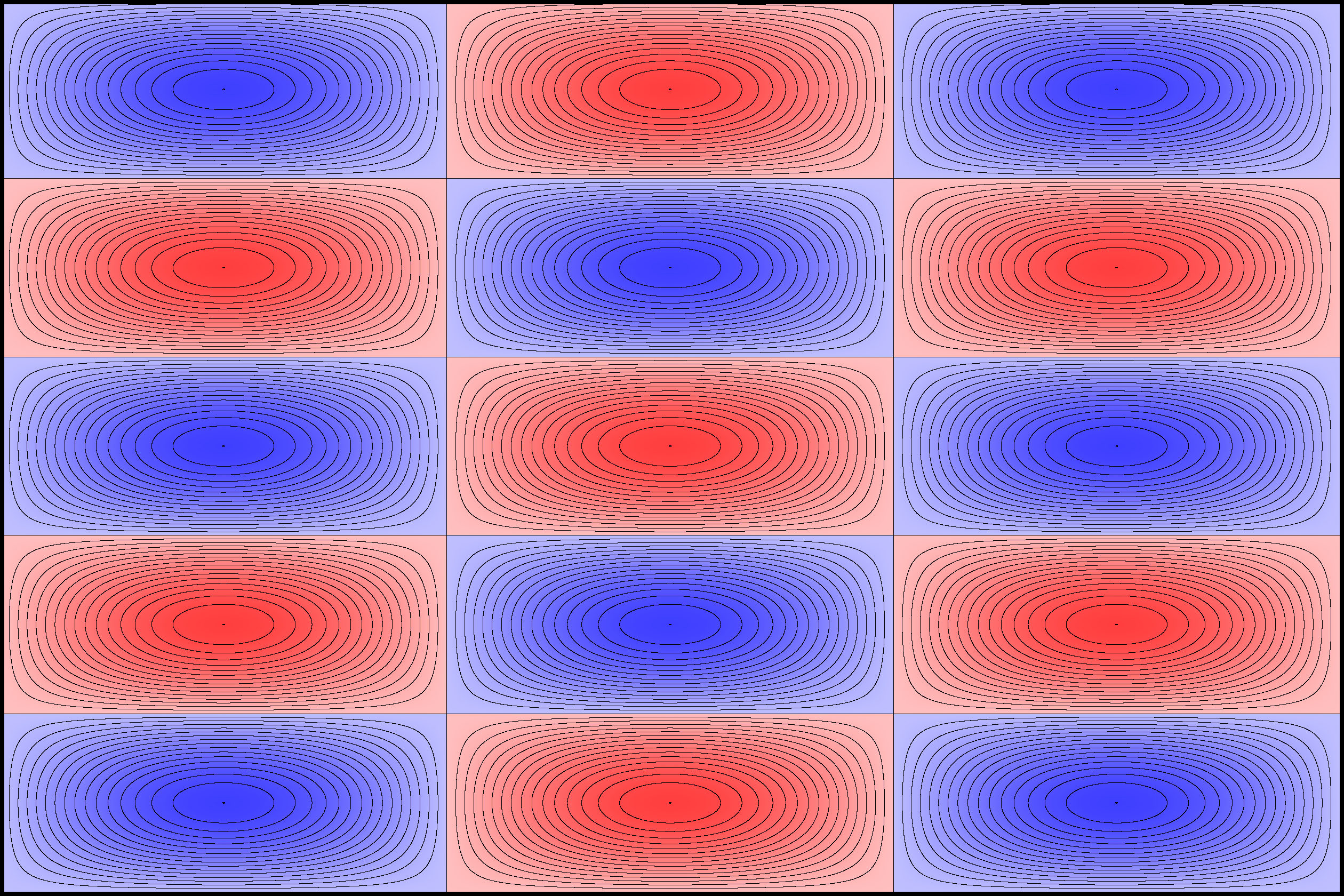
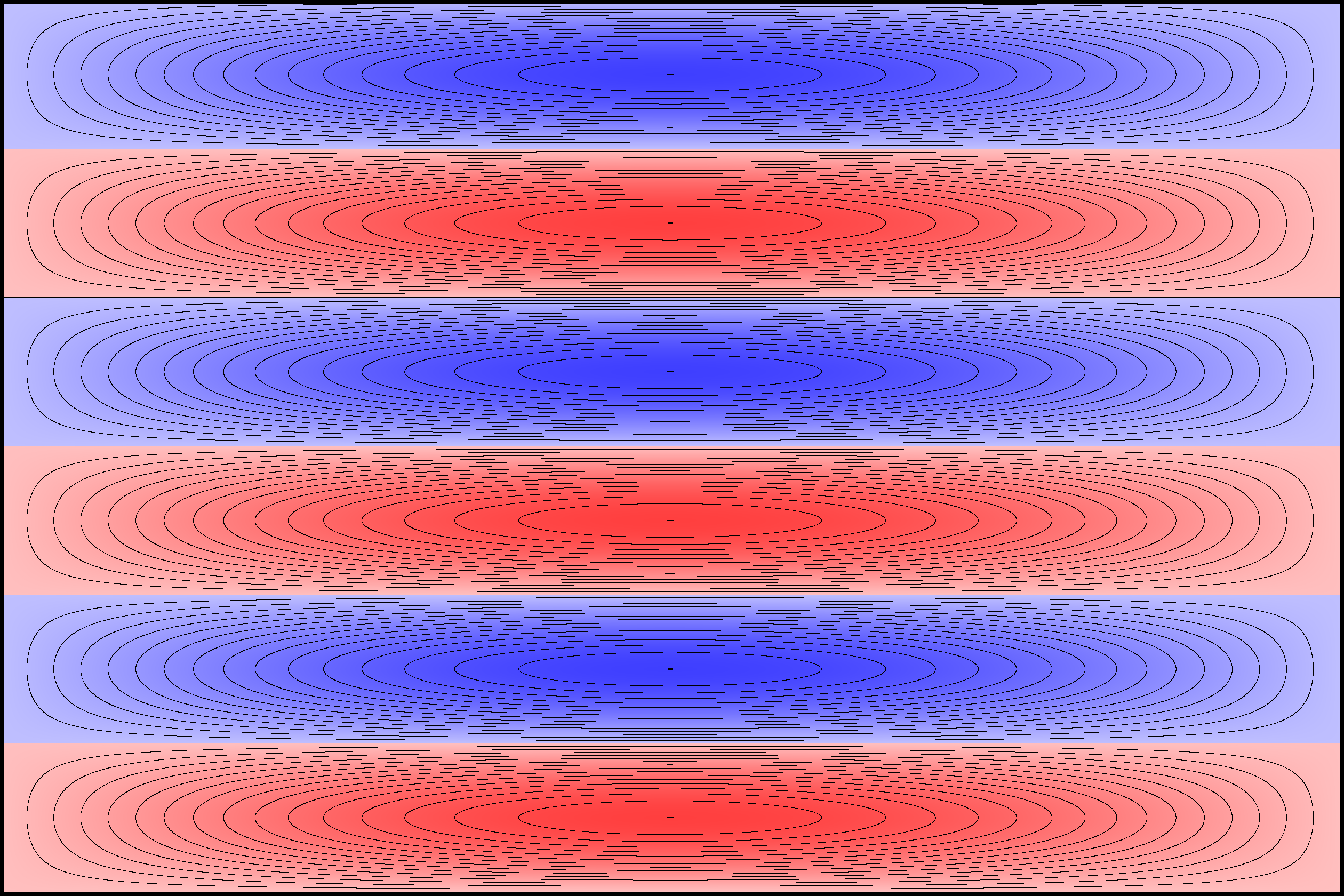
Rectangular plates are much less interesting, here's 2x1:

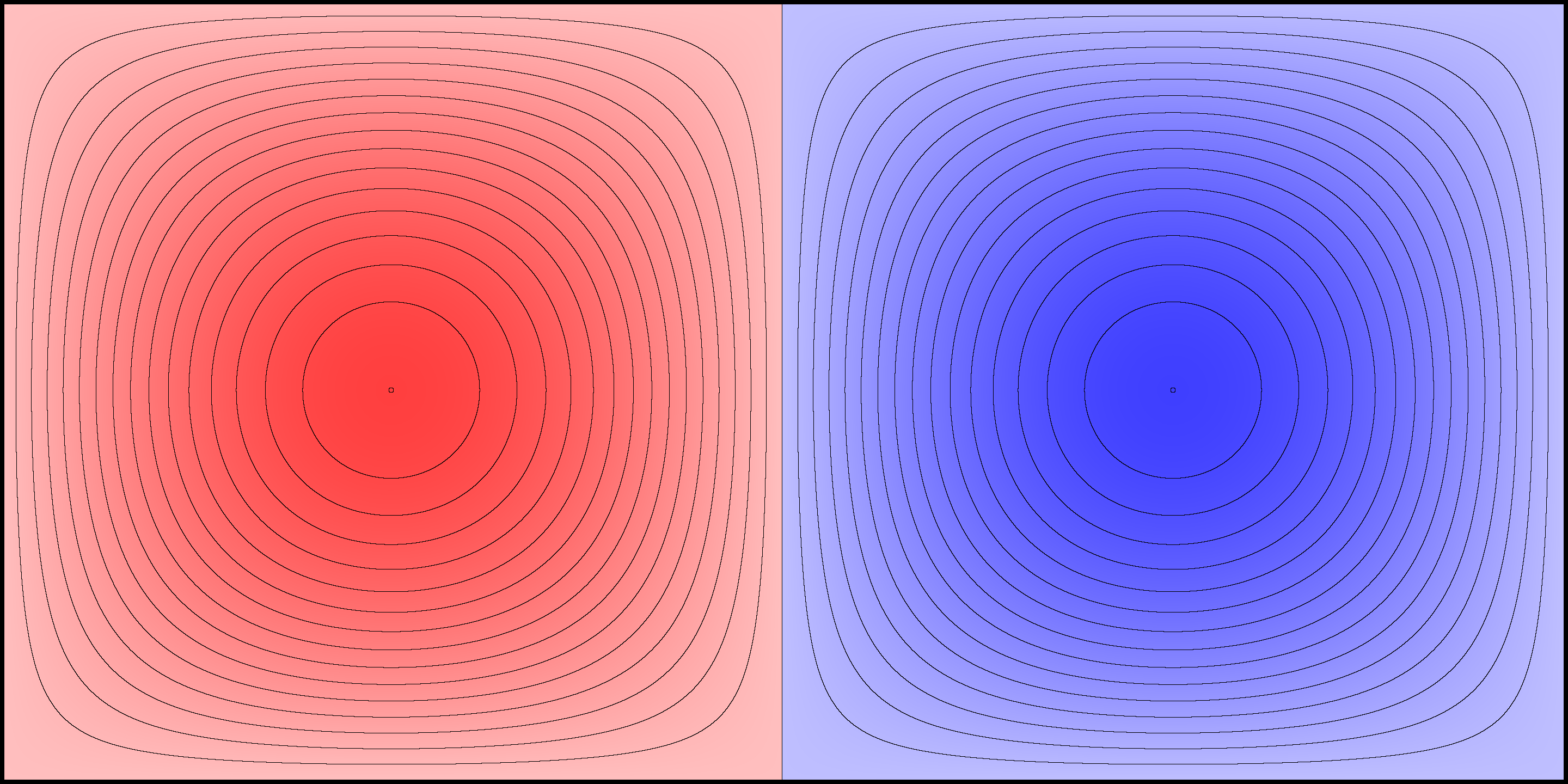
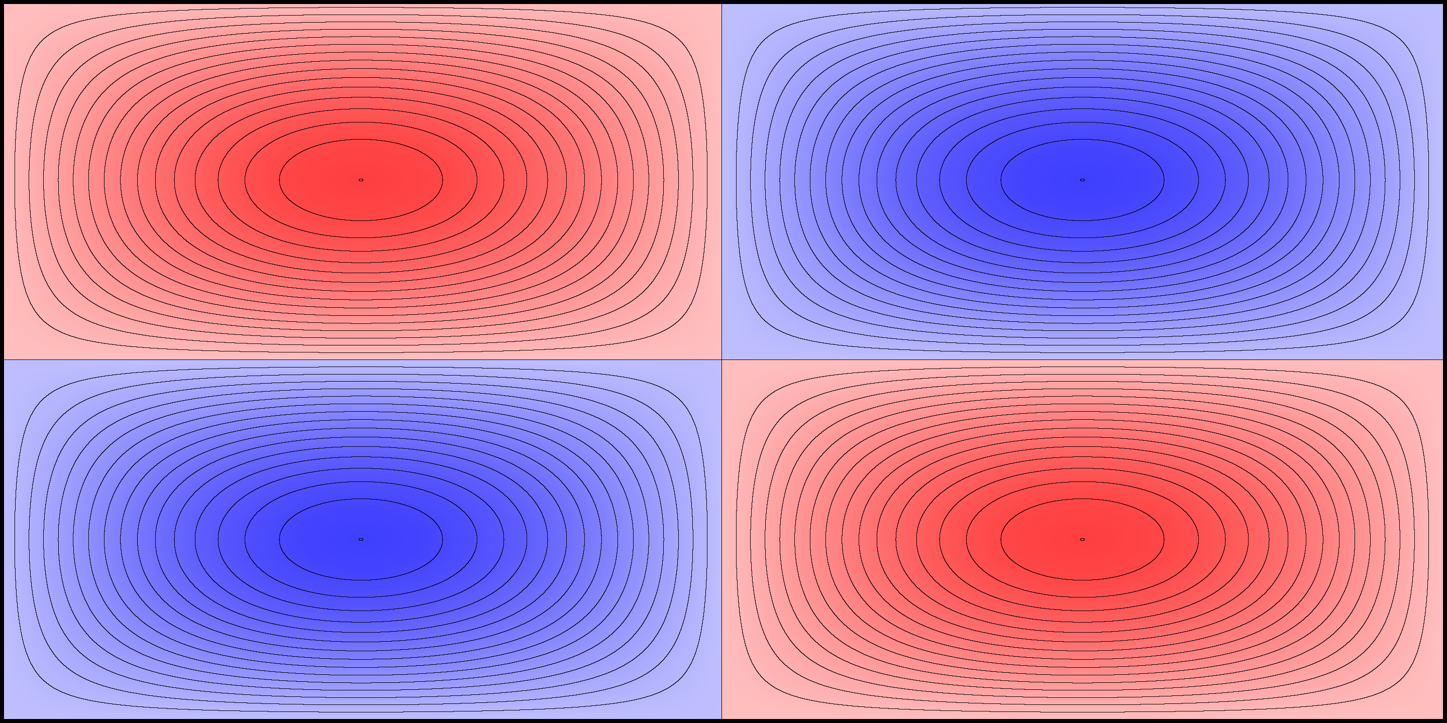
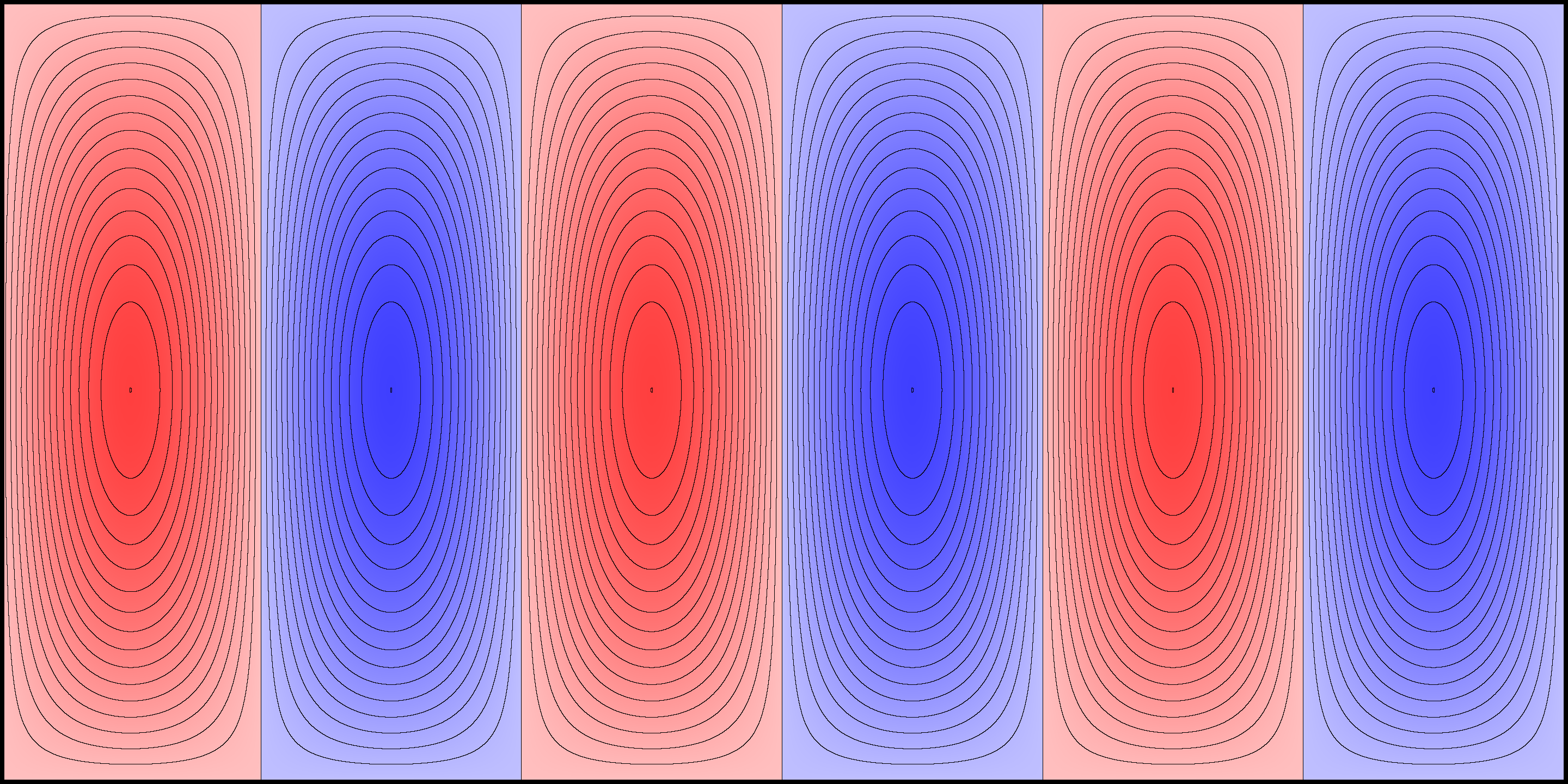
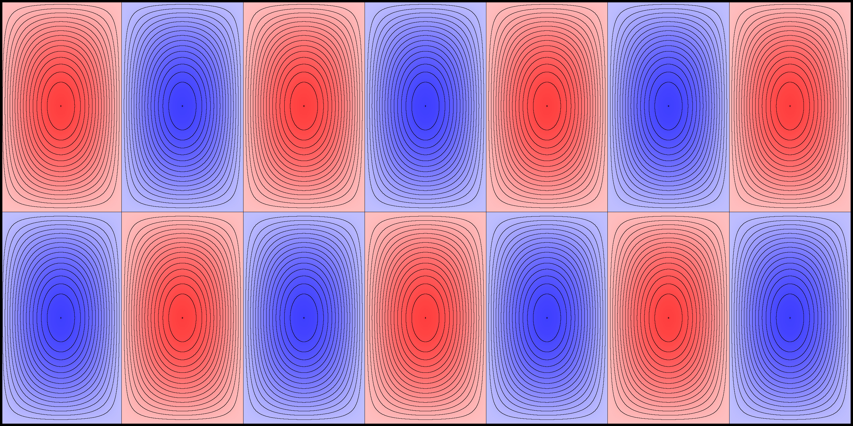
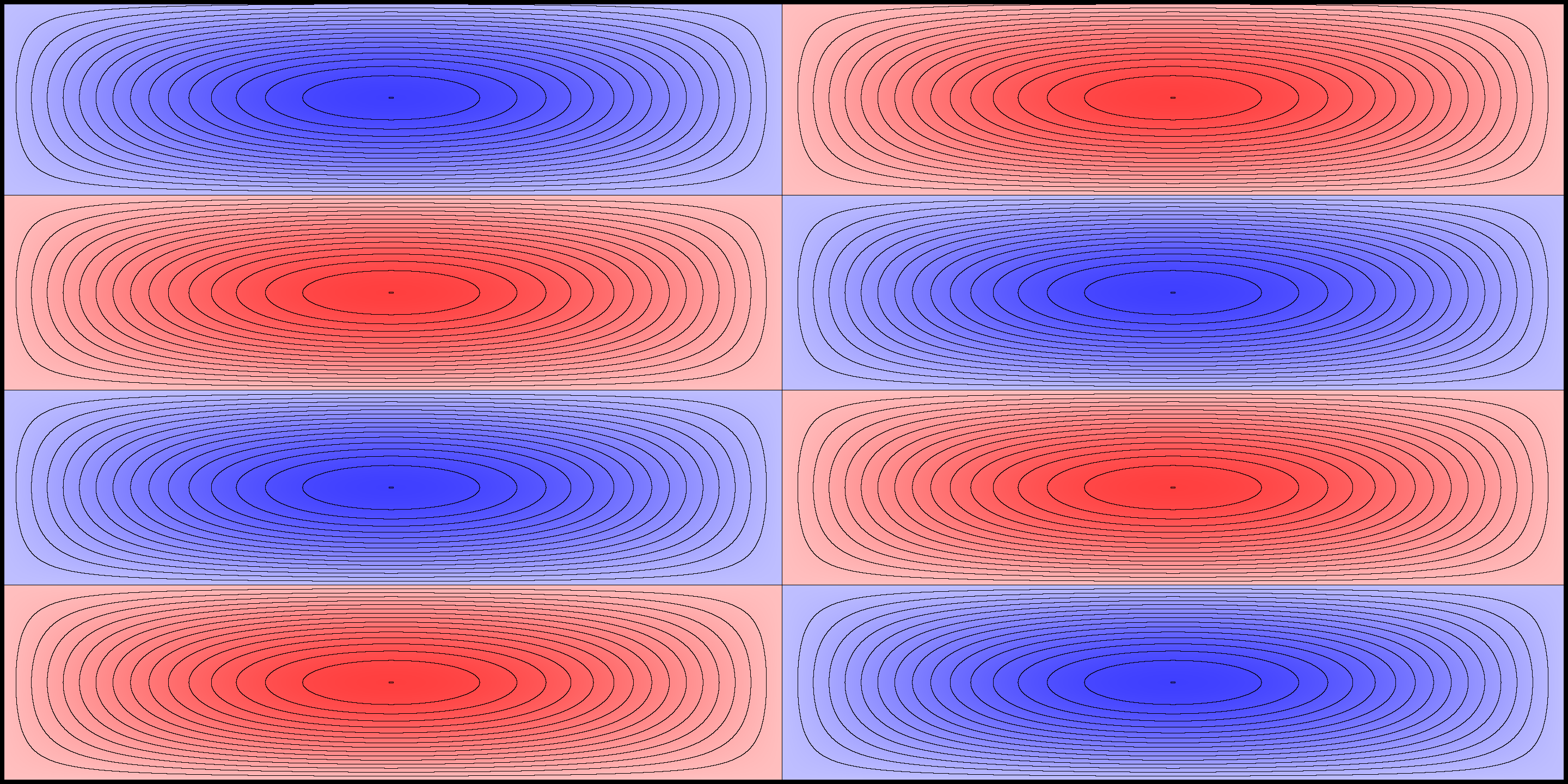
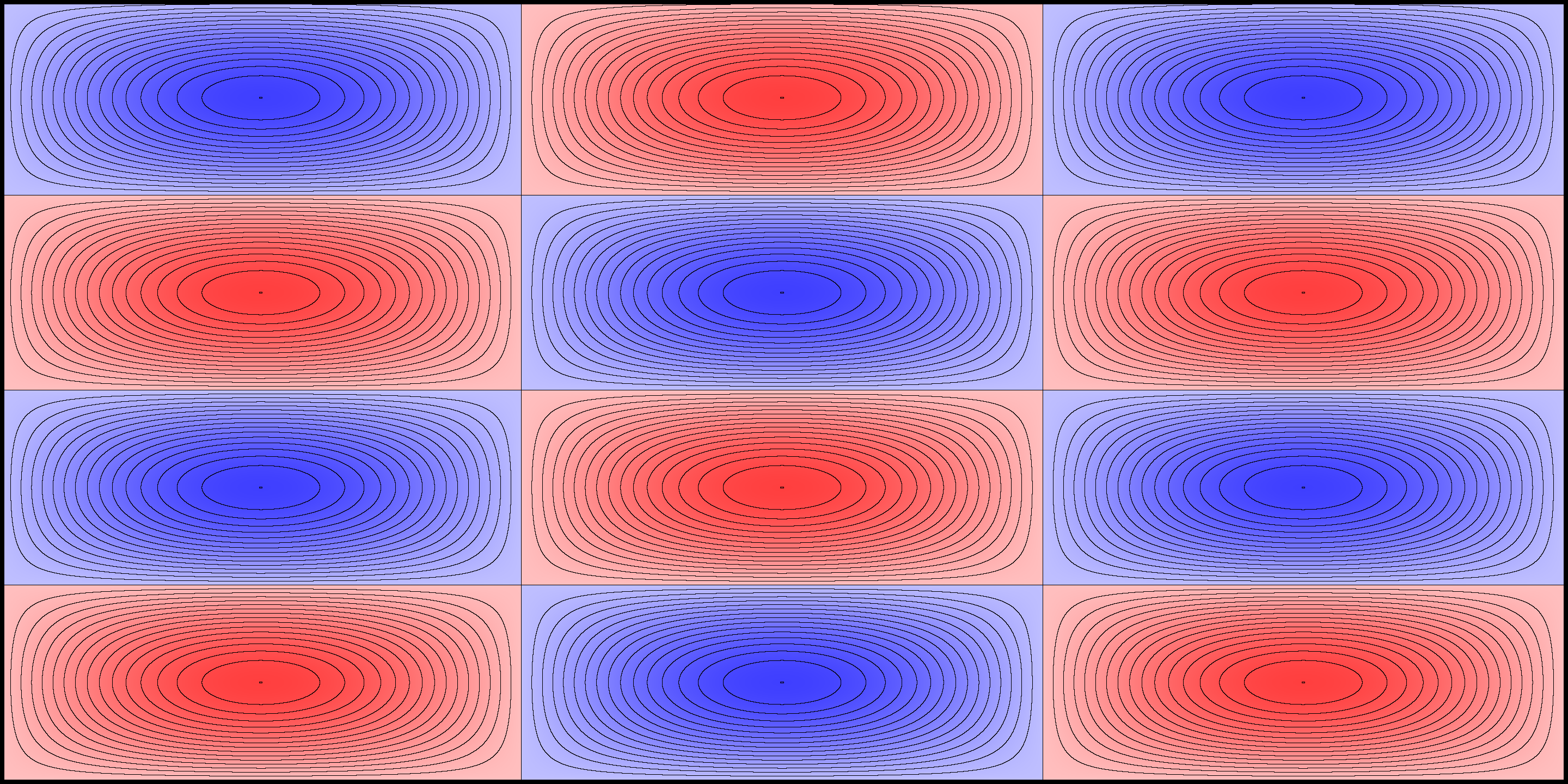
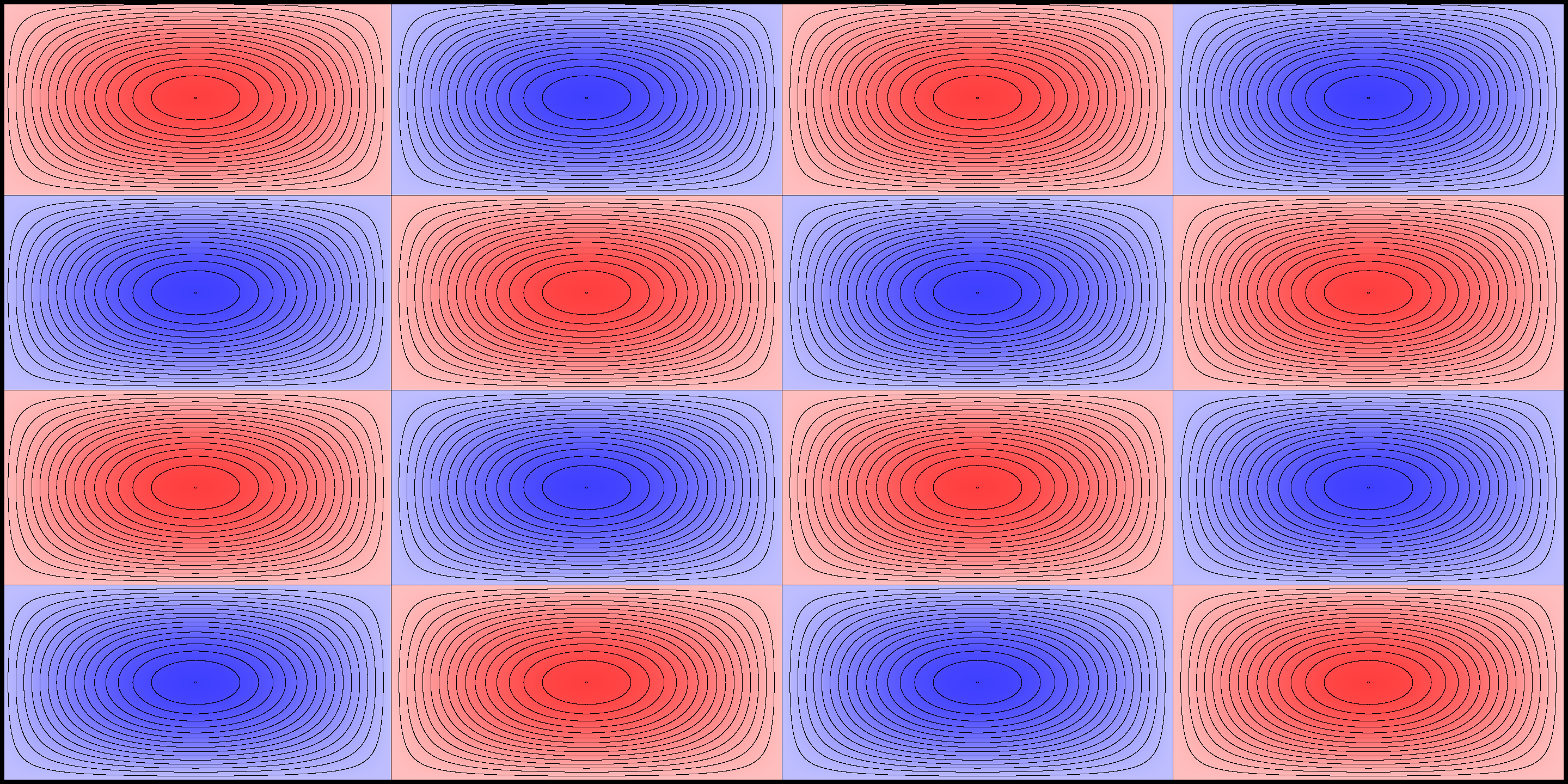
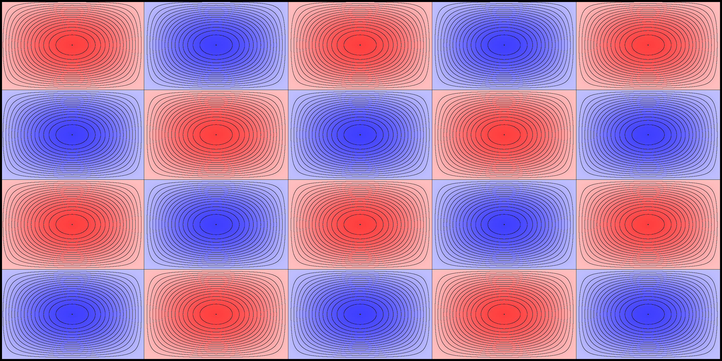
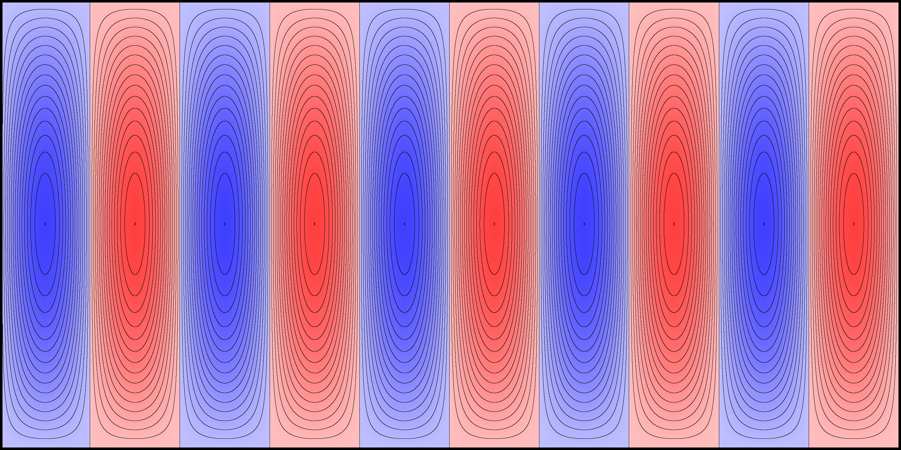
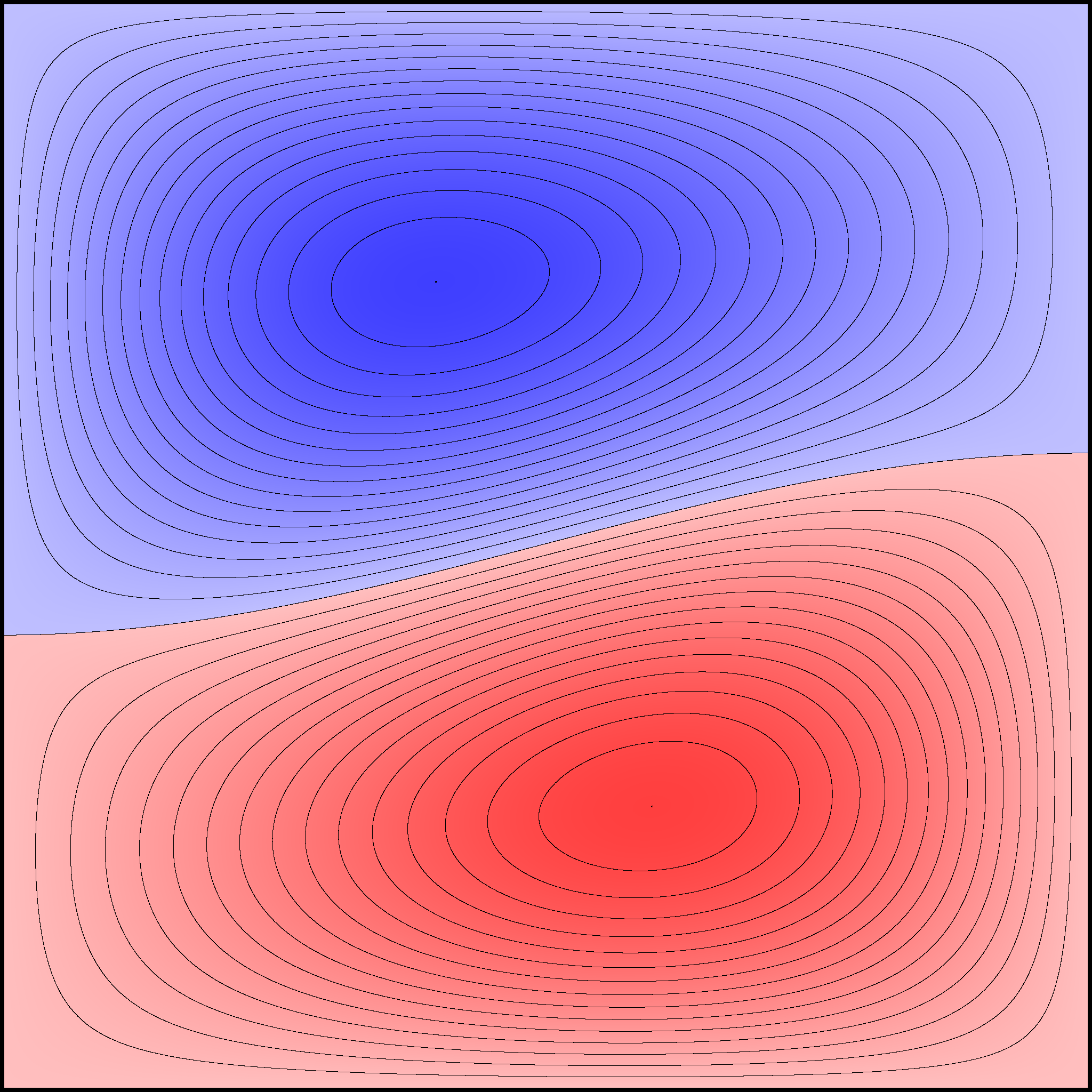
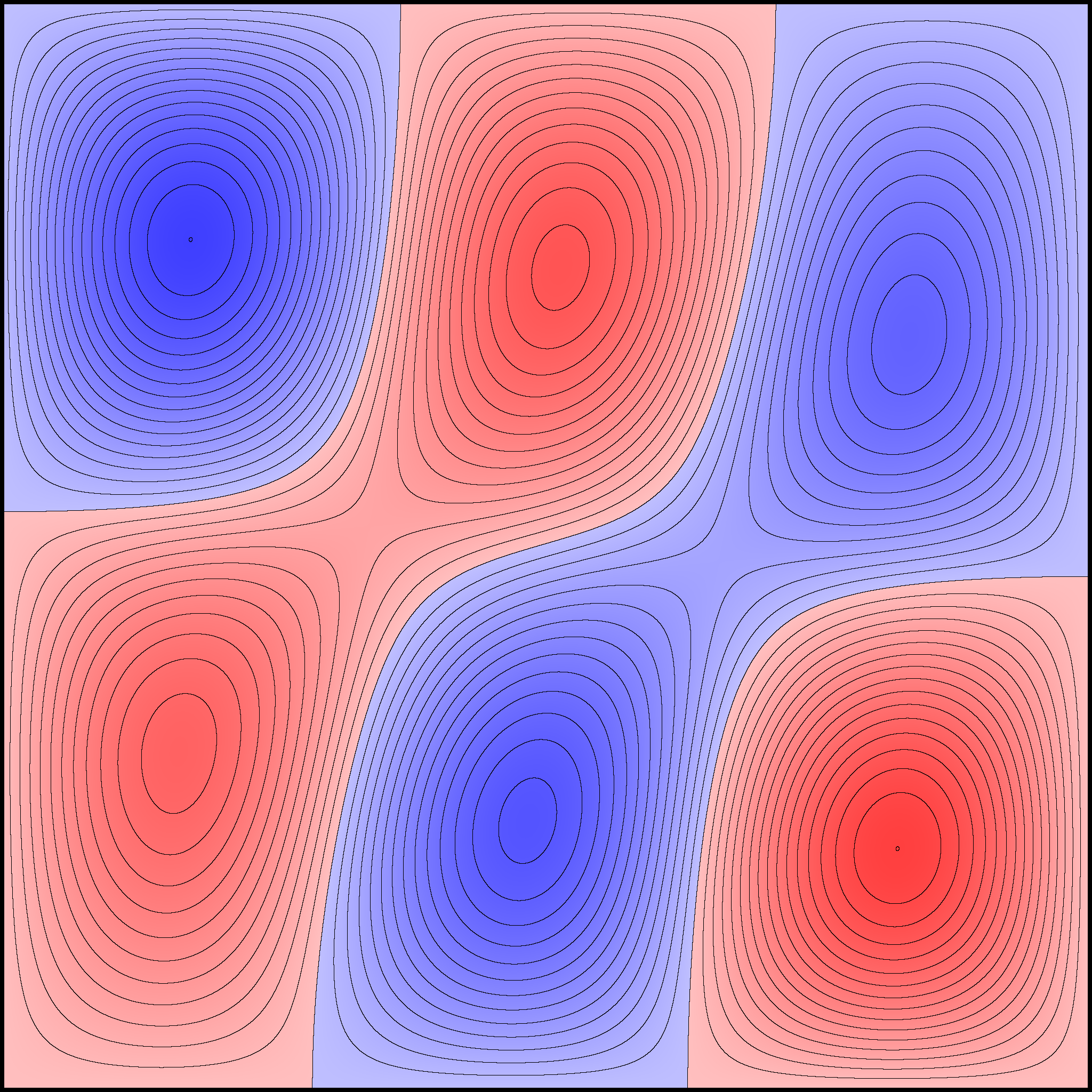
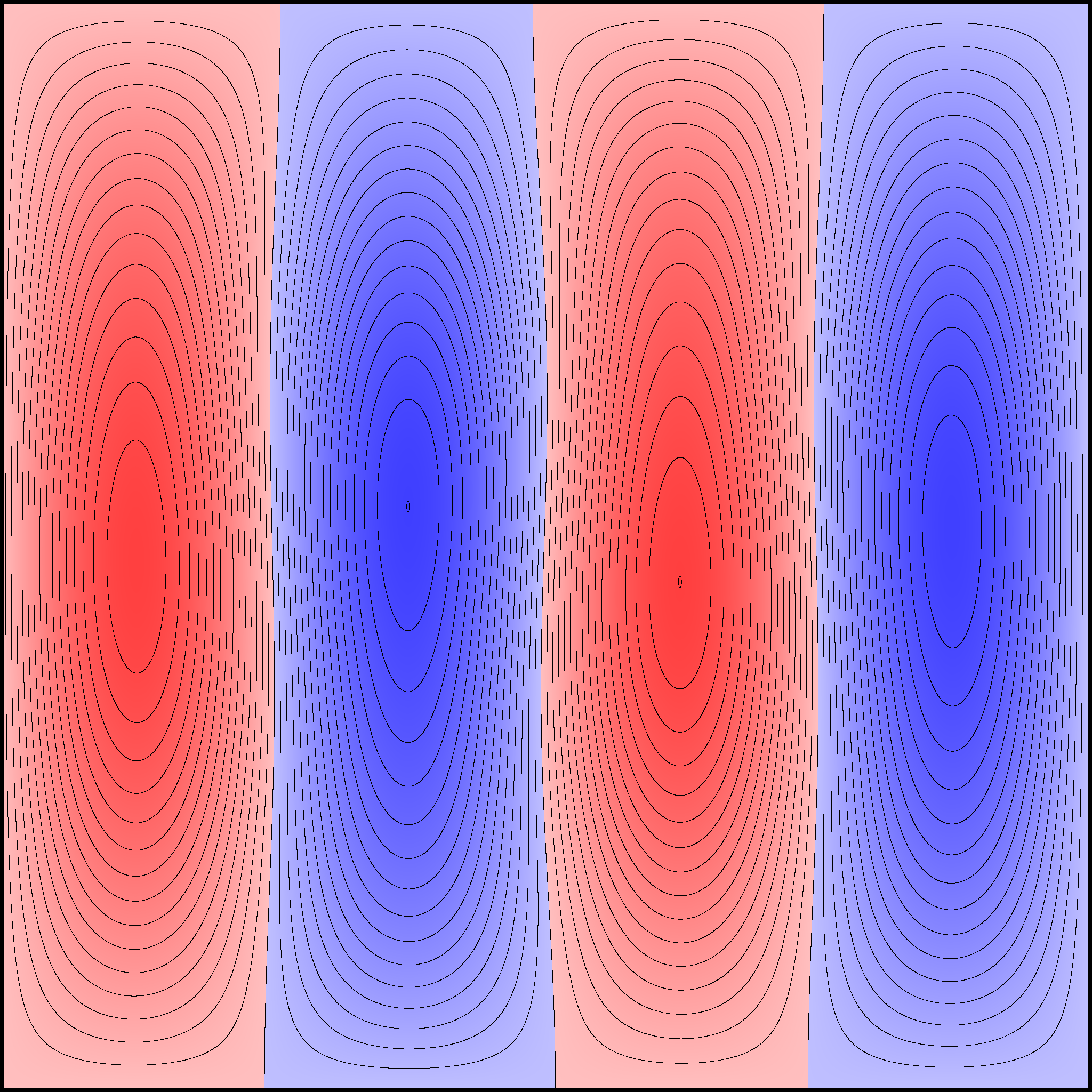
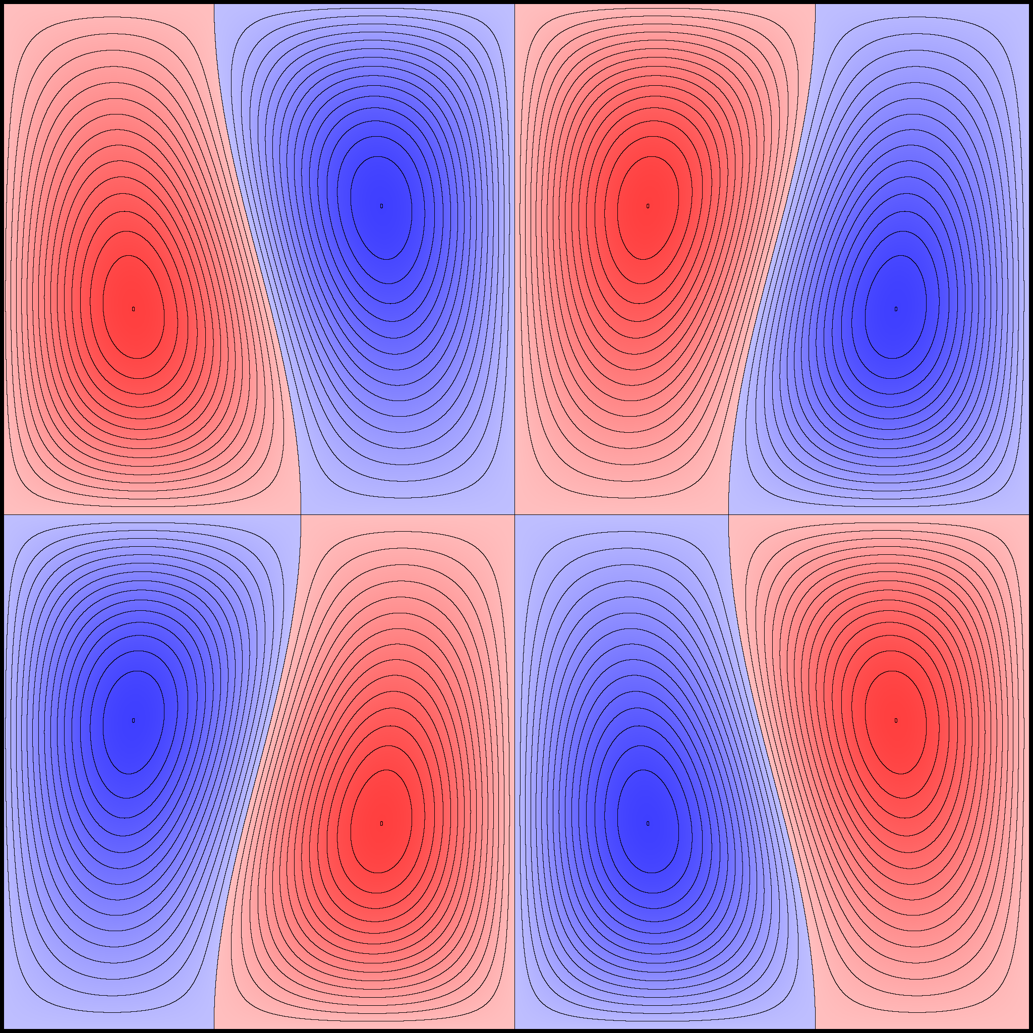
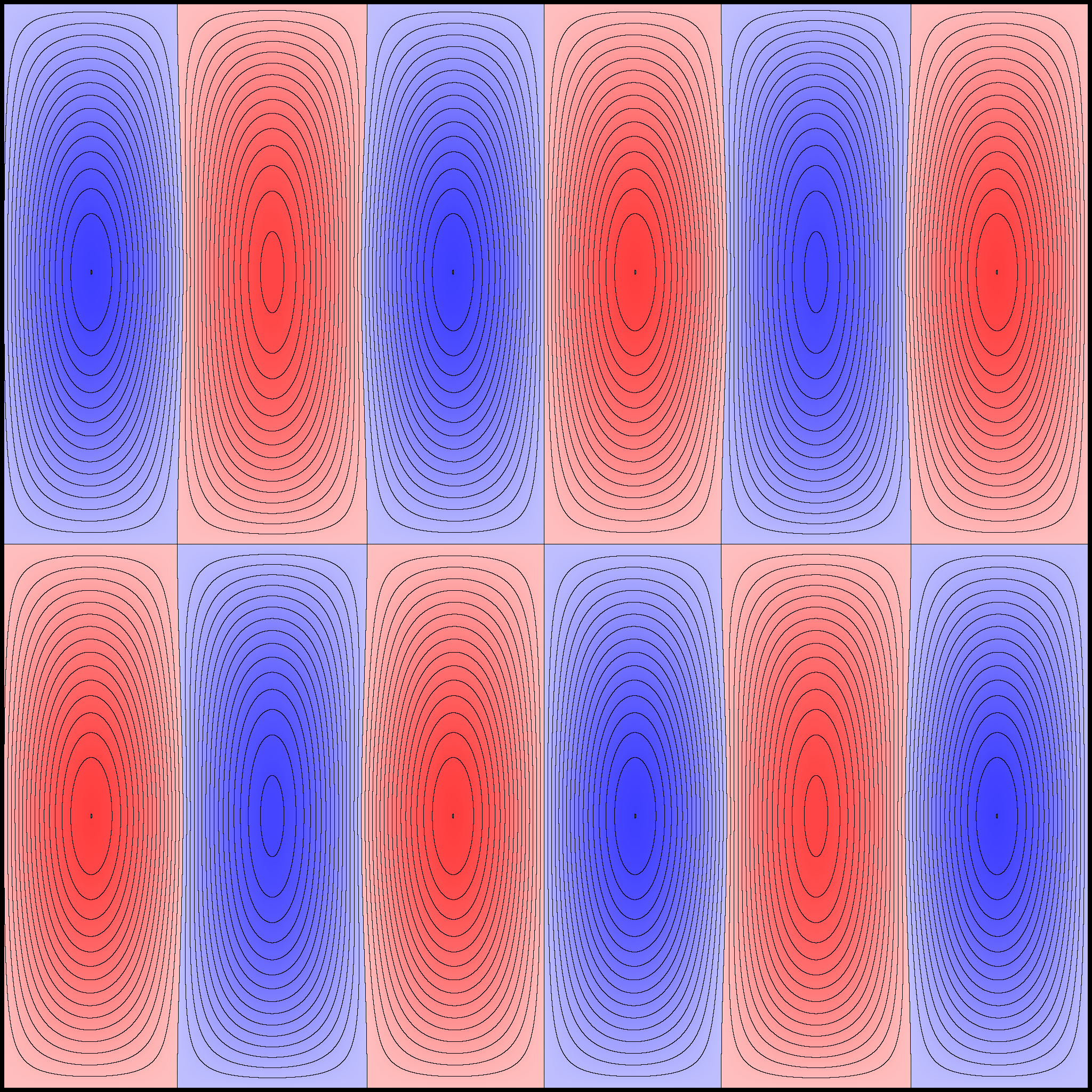
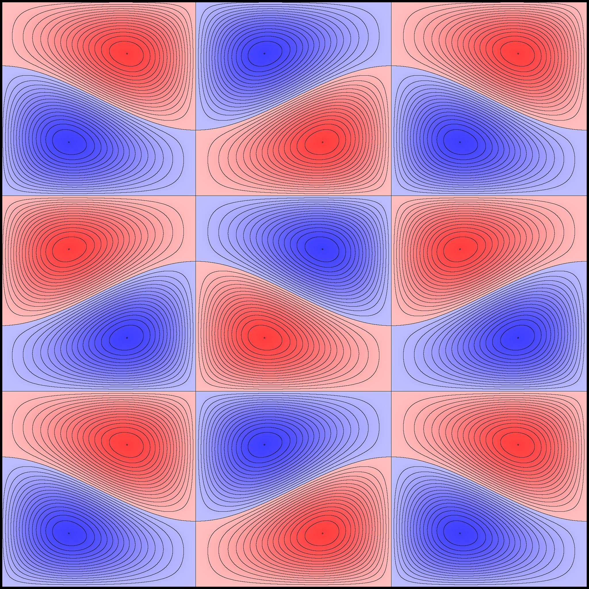
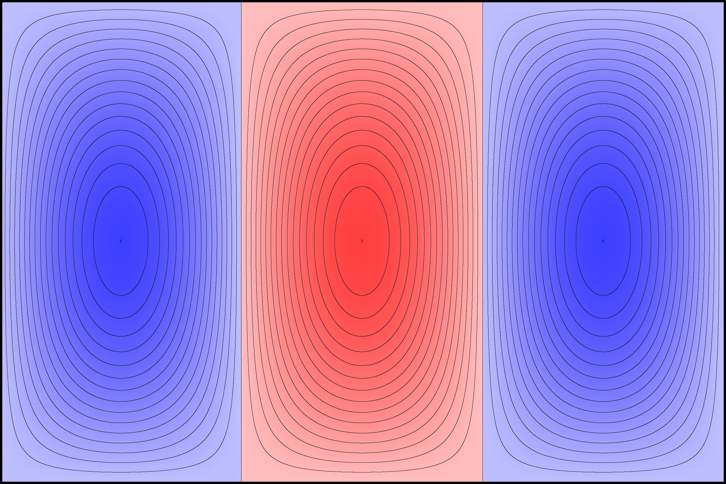
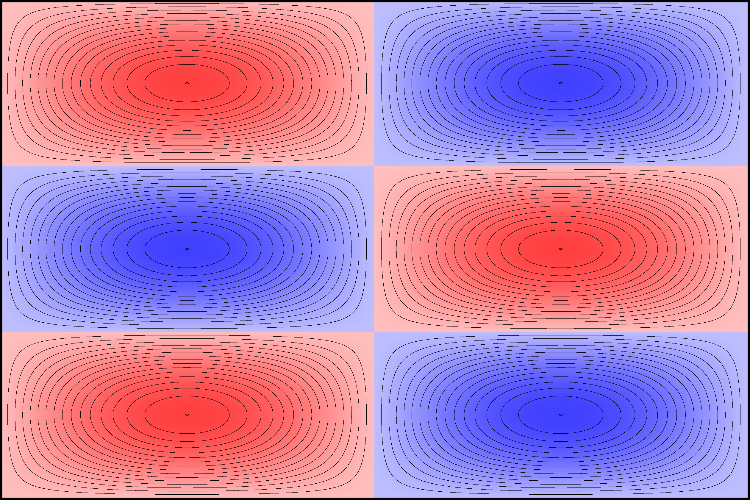
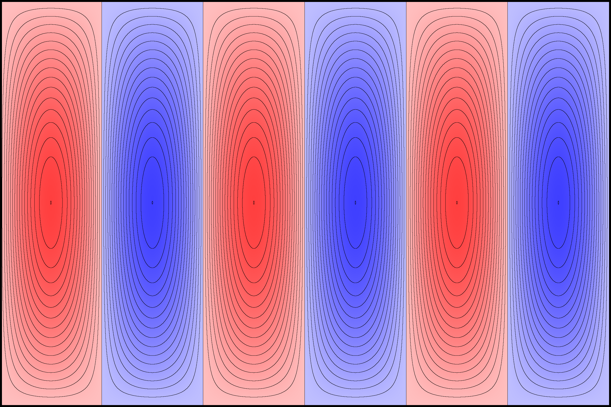
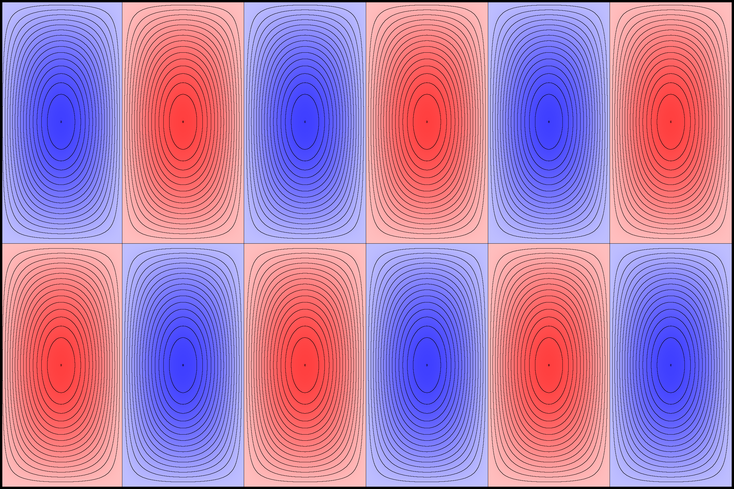
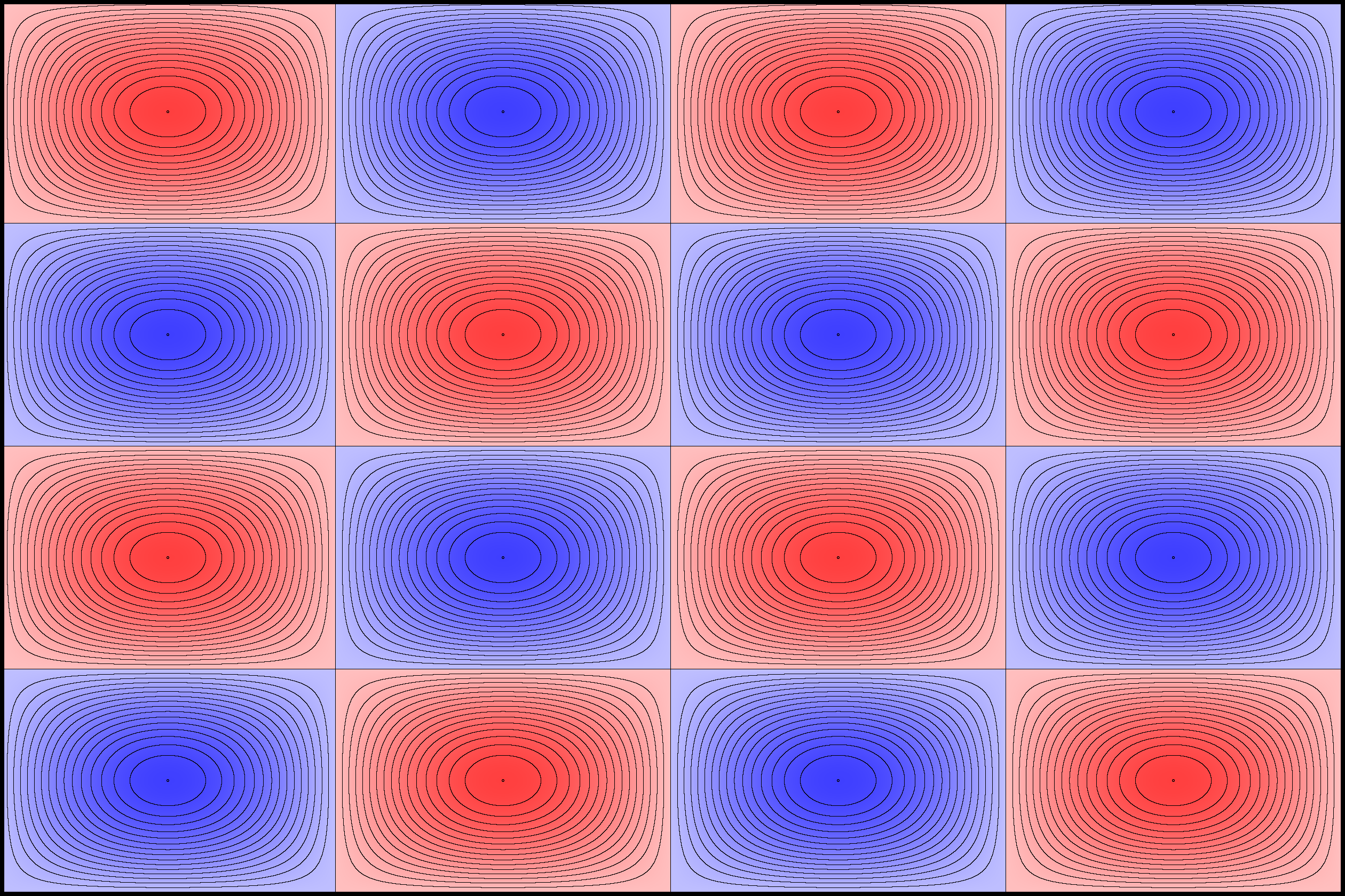
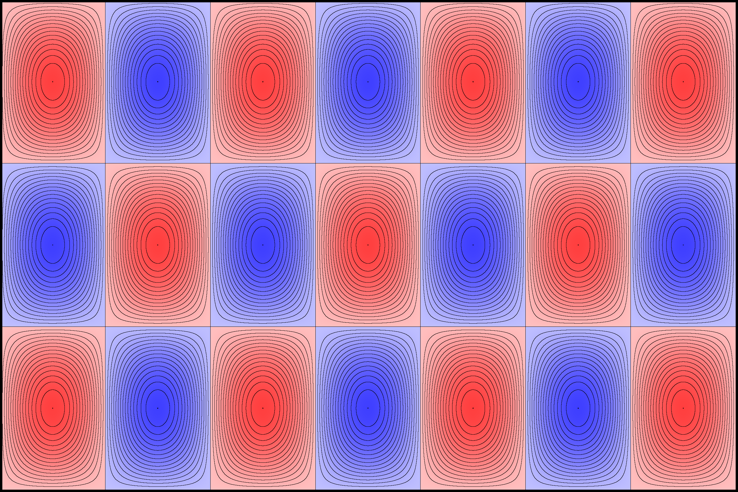
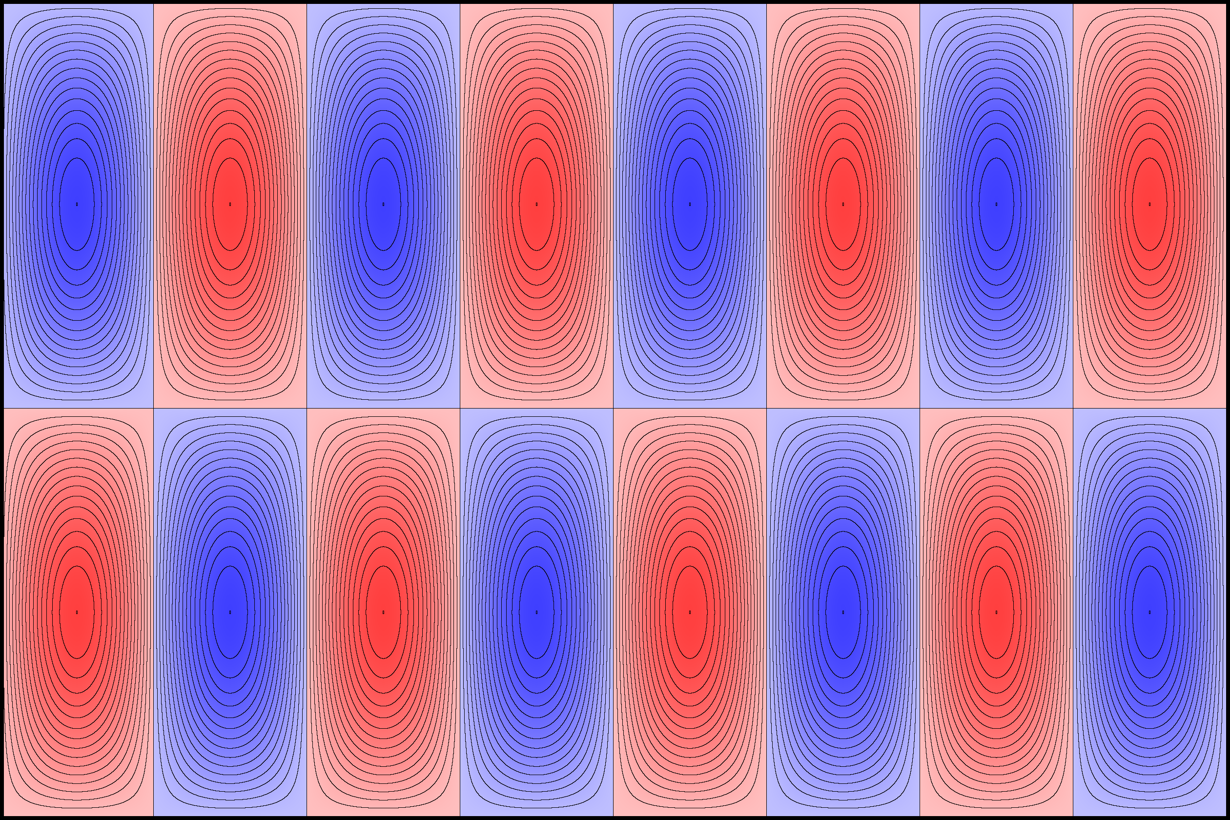
And 3x2:

Source code downloads:

modes.m

GNU Octave source to generate and solve a sparse eigensystem, outputs raw data.

modes.c

C99 source to take the raw data and turn it into pretty pictures.

Each source has hardcoded values (e, m, n) near the top, these must match across both files or bad things will happen.