# Quadtree Filter
Kurbitur described an algorithm for adaptive image pixelation with an implementation in Python: Quadtree Image Filter.
Other prior art includes: Quads.
The main idea: if a region has high variance, subdivide it and recurse on the pieces, otherwise, fill the region with its mean. Each channel is processed independently.
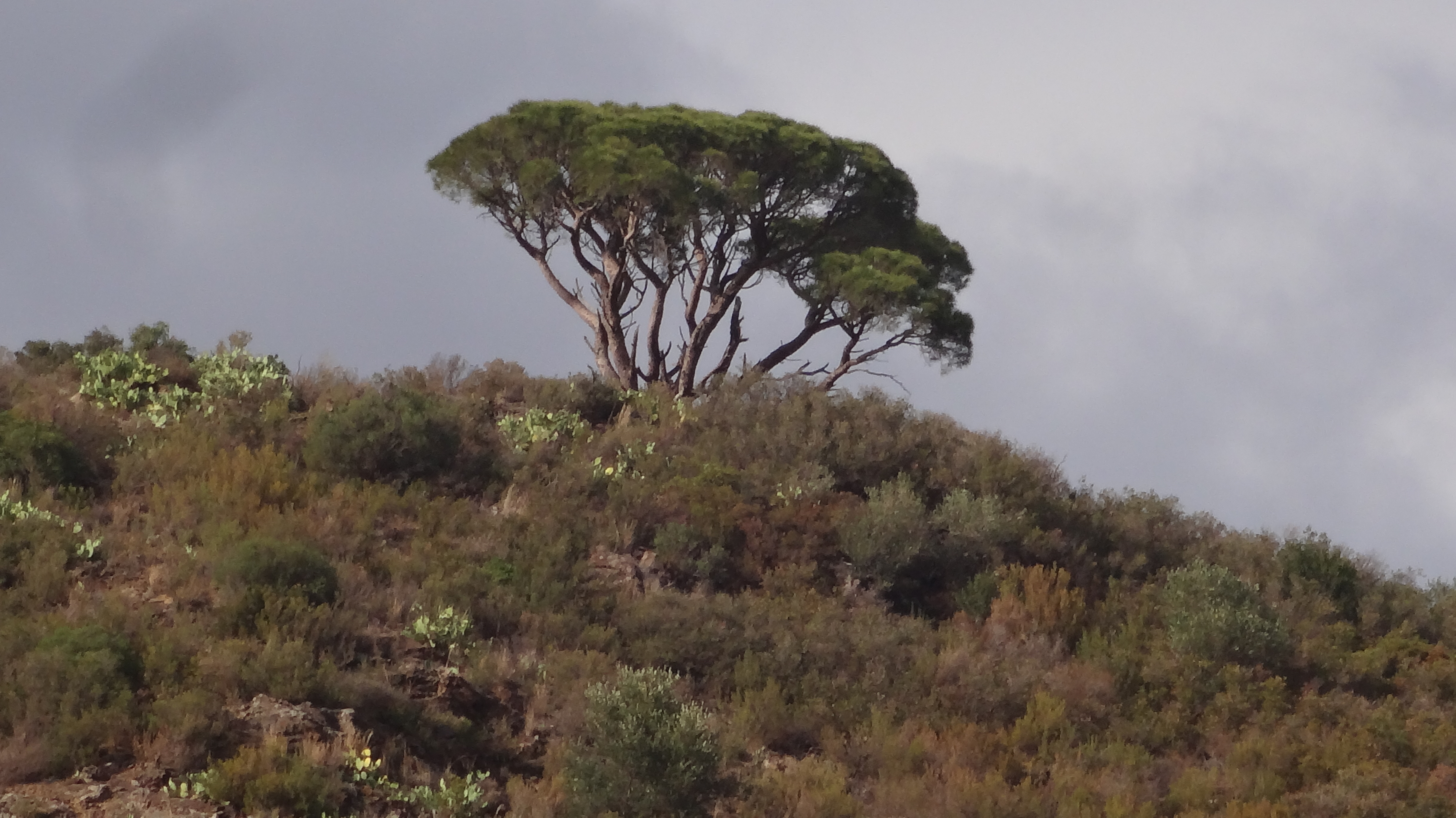
# 1 Example
Input:
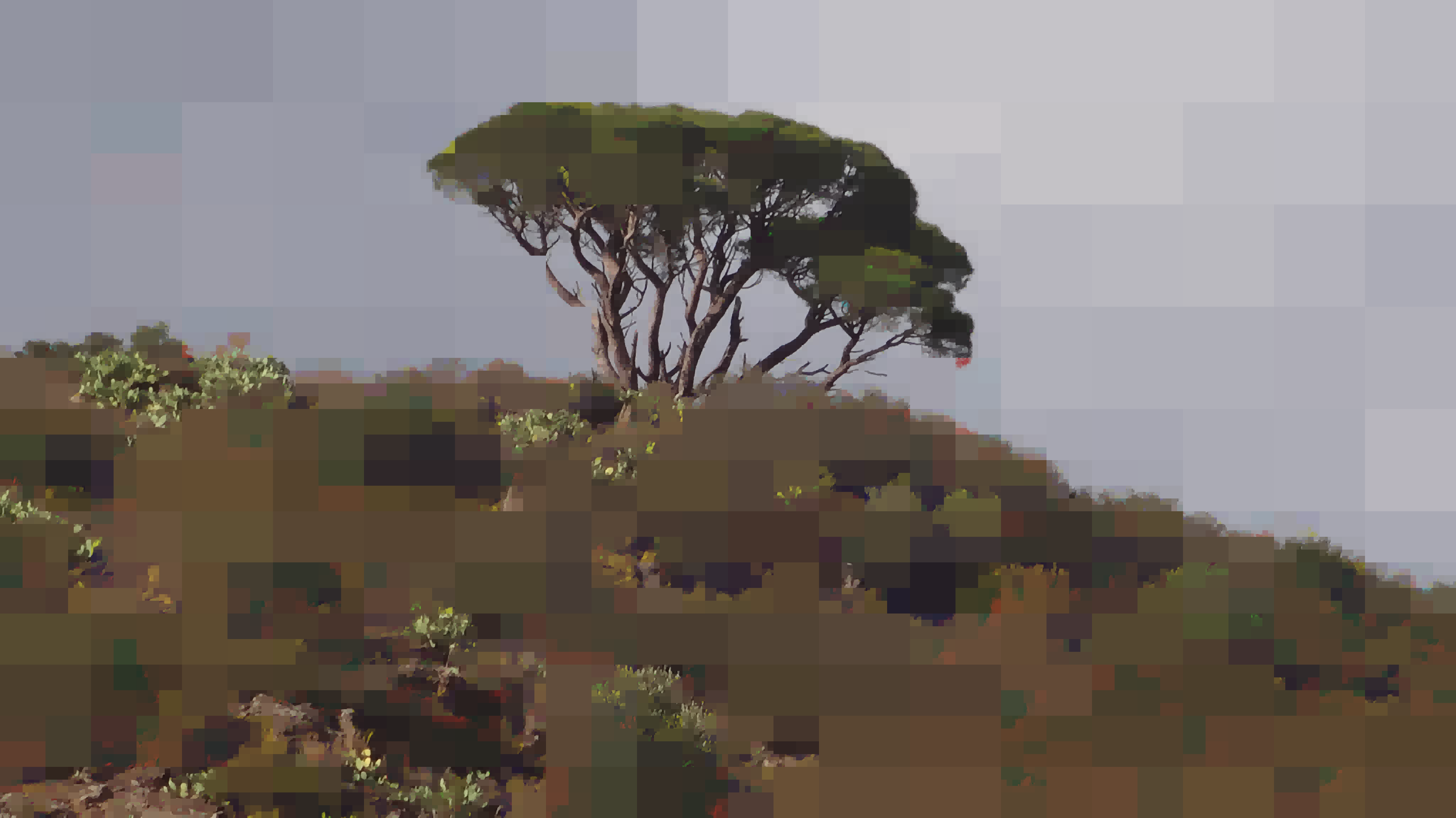
Output (threshold 15):
# 2 Implementation
I used the C programming language with summed-area table data structure to (hopefully) accelerate variance computations.
Download: quadtree-filter.c.
# 3 Video
Video could be processed either frame by frame independently, or with summed-volume tables, but memory costs for the latter are probably prohibitive beyond short clips, and the relative weighting between horizontal+vertical and time axes might need to be adjustable for different frame rates.
# 4 Efficiency
Computation time depends on how the image is subdivided, which depends on the variance threshold parameter and the particular image being processed.
# 4.1 Worst Case
Consider the worst case, where each pixel is unique. This means four divisions at each level.
In a simple implementation with recomputation, computing the variances at level \(L\) takes \((W \times H + 4^{L + 1})\) multiplications, \((W \times H \times 2 + 4^{L})\) additions, and \((W \times H)\) memory accesses. Because the deepest level has \(4^L = W \times H\), and the series is geometric, this works out to about \(\frac{16}{3} + \log_4 (W \times H)\) multiplications per pixel, \(\frac{4}{3} + 2 \log_4 (W \times H)\) additions per pixel, and \(\frac{4}{3} \log_4 (W \times H)\) memory accesses per pixel.
With summed area tables, the preprocessing step takes \(1\) multiplication per pixel, \(4\) additions per pixel, and \(5\) memory accesses per pixel. Then computing the variances at level \(L\) takes \(4^{L + 1}\) multiplications, \(7 \times 4^L\) additions, and \(4 \times 4^L\) memory accesses (originally I had \(8\), but the previous level’s memory accesses can be reused). This works out to total about \(\frac{19}{3}\) multiplications per pixel, \(\frac{40}{3}\) additions per pixel, and \(\frac{31}{3}\) memory accesses per pixel.
Comparing the two implementations, the number of multiplications is equal for \(2 \times 2\) images, the number of additions is equal for \(64 \times 64\) images, and the number of memory accesses is equal for \(2896 \times 2896\) images. If cost is (arbitrarily) multiplications plus additions plus memory accesses, the cost would be equal at image size \(42 \times 42\).
So overall, using summed-area tables is likely a big win, because cost per pixel is constant, while cost per pixel for simple recomputation goes up with image size.
# 4.2 Good Case
Suppose in a good case that only half the active regions are subdivided.
Then simple costs reduce: computing the variances at level \(L\) takes \((\frac{W \times H}{2^L} + 2^{L + 1})\) multiplications, \((\frac{W \times H}{2^L} \times 2 + 2^{L})\) additions, and \((\frac{W \times H}{2^L})\) memory accesses. This works out to about \(2\) multiplications per pixel, \(4\) additions per pixel, and \(2\) memory accesses per pixel.
Meanwhile summed area table preprocessing costs are unchanged, Then computing the variances at level \(L\) takes \(2^{L + 1}\) multiplications, \(7 \times 2^L\) additions, and \(4 \times 2^L\) memory accesses. Total costs are completely dominated by the preprocessing, i.e., \(1\) multiplication per pixel, \(4\) additions per pixel, and \(5\) memory accesses per pixel.
Now both costs are constant per pixel, nothing too conclusive about which method is best in this case.