mathr / blog / #

I recently came across Arnaud Chéritat's polynomial mating movies and just had to try to recreate them.

If \(p\) and \(q\) are in the Mandelbrot set, they have connected Julia sets for the quadratic polynomial functions \(z^2+p\) and \(z^2+q\). If they are not in conjugate limbs (a limb is everything beyond the main period 1 cardioid attached at the root of a given immediate child bulb, conjugation here is reflection in the real axis, the 1/2 limb is self-conjugate) then the Julia sets can be mated: glue the Julia sets together respecting external angles so that the result fills the complex plane (which is conveniently represented as the Riemann sphere). It turns out that this mating is related to the Julia set of a rational function of the form \(\frac{z^2+a}{z^2+b}\).

One algorithm to compute \(a\) and \(b\) is called "slow mating". Wolf Jung has a pre-print which explains how to do it in chapter 5: The Thurston Algorithm for quadratic matings.

My first attempts just used Wolf Jung's code and later my own code, to compute the rational function and visualize it in Fragmentarium (FragM fork). This only worked for displaying the final limit set, while Chéritat's videos had intermediate forms. I found a paper which had this to say about it:

On The Notions of Mating

Carsten Lunde Petersen & Daniel Meyer

5.4. Cheritat movies

It is easy to see that \(R_\lambda\) converges uniformly to the monomial \(z^d\) as \(\lambda \to \infty\). Cheritat has used this to visualize the path of Milnor intermediate matings \(R_\lambda\), \(\lambda \in ]1,\infty[\) of quadratic polynomials through films. Cheritat starts from \(\lambda\) very large so that \(K_w^\lambda\) and \(K_b^\lambda\) are essentially just two down scaled copies of \(K_w\) and \(K_b\), the first near \(0\), the second near \(\infty\). From the chosen normalization and the position of the critical values in \(K_w^\lambda \cup K_b^\lambda\) he computes \(R_\sqrt{\lambda}\). From this \(K_w^\sqrt{\lambda} \cup K_b^\sqrt{\lambda}\) can be computed by pull back of \(K_w^\lambda \cup K_b^\lambda\) under \(R_\sqrt{\lambda}\). Essentially applying this procedure iteratively one obtains a sequence of rational maps \(R_{\lambda_n}\) and sets \(K_w^{\lambda_n} \cup K_b^{\lambda_n}\), where \(\lambda_n \to 1+\) and \(\lambda_n^2 = \lambda_{n-1}\). For more details see the paper by Cheritat in this volume.

What seems to be the paper referred to contains this comment:

Tan Lei and Shishikura’s example of non-mateable degree 3 polynomials without a Levy cycle

Arnaud Chéritat

Figure 4

The Riemann surface \(S_R\) conformally mapped to the Euclidean sphere, painted with the drawings of Figure 2. The method for producing such a picture is interesting and will be explained in a forthcoming article; it does not work by computing the conformal map, but instead by pulling-back Julia sets by a series of rational maps. It has connections with Thurston's algorithm.

I could not find that "forthcoming" article despite the volume having been published in 2012 following the 2011 workshop, so I emailed Arnaud Chéritat and got a reply to the effect that it had been cancelled by the author.

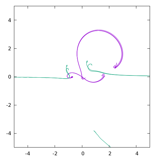
My first attempts at coding the slow mating algorithm worked by pulling back the critical orbits as described in Wolf Jung's preprint. The curves look something like this:

A little magic formula for finding the parameters \((a, b)\) for the function \(\frac{z^2+a}{z^2+b}\):

\[a = \frac{C(D-1)}{D^3(1-C)}\] \[b = \frac{D-1}{D^2(1-C)}\]

where \((C,D)\) are the pulled back \(1\)th iterates. This was reverse-engineered from Wolf Jung's code, which worked with separate real and imaginary components, with no comments and heavy reuse of the same variable names. I'm not sure if it is correct but it seems to give useable results when plugged into FragM for visualization:

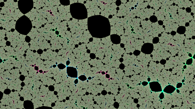
I struggled to implement the intermediate images at first: I tried pulling back from the coordinates of a filled in Julia set but that needed huge amounts of memory and the resolution was very poor:

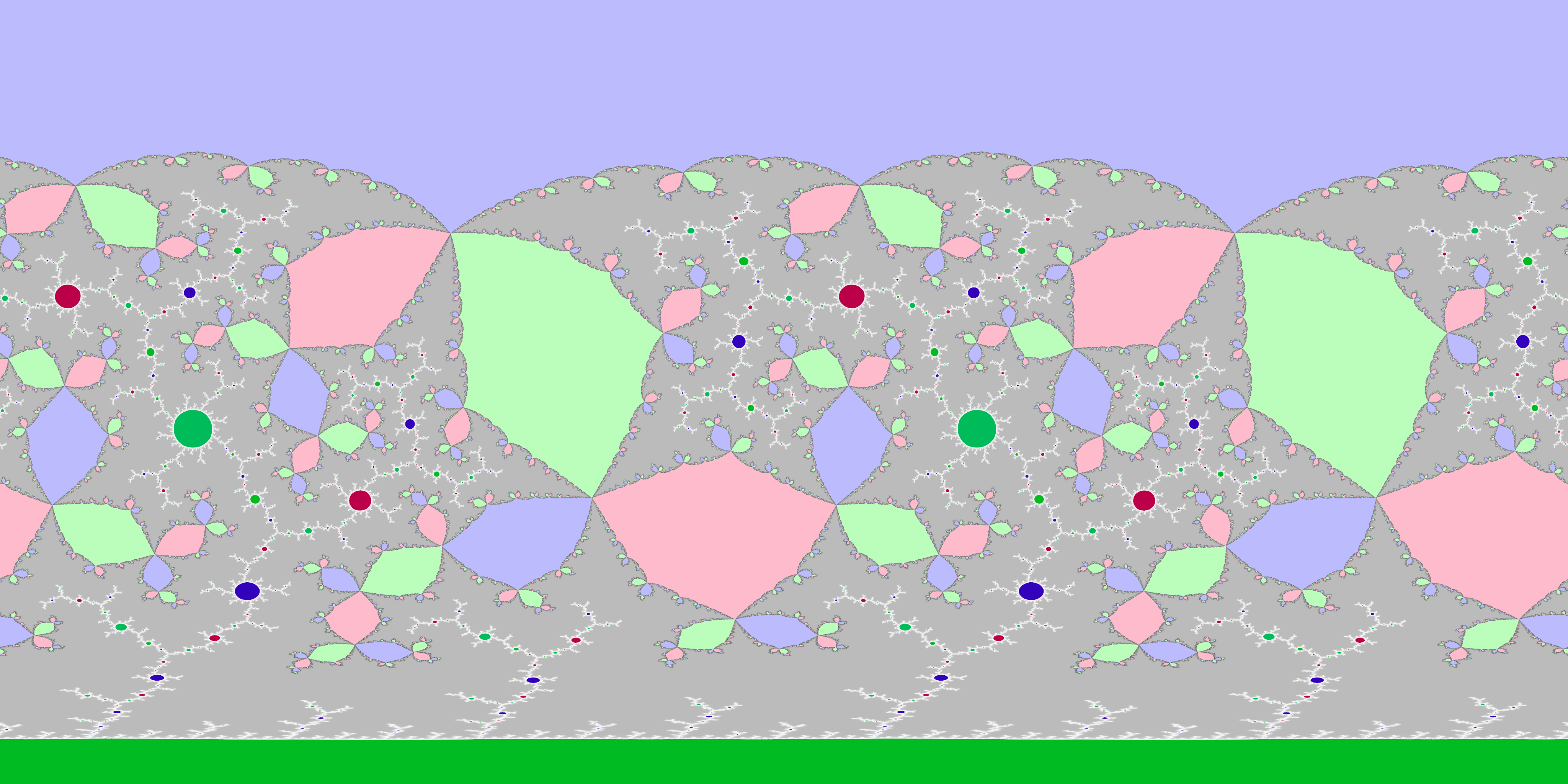
Eventually I figured out that I could invert each pullback function into something of the form \(\frac{az^2+b}{cz^2+d}\) and push forward from pixel coordinates to colour according to which hemisphere it reached:

I struggled further, until I found the two bugs that were almost cancelling each other out. The coordinates in each respective hemisphere can be rescaled, and thereafter regular iterations of \(z^2+c\) until escape or maximum iterations could be used to colour the filled in Julia sets expanding within each hemisphere:

After that it was quite simple to bolt on dual-complex-numbers for automatic differentiation, to compute the derivatives for distance estimation to make the filaments of some Julia sets visible:

I also added an adaptive super-sampling scheme: if the standard deviation of the current per-pixel sample population divided by the number of samples is less than a threshold, I assume that the next sample will make negligible changes to the appearance, and so I stop. This speeds up interior regions (which need to be computed to the maximum iteration count) because the standard deviation will be 0 and it will stop after only the minimum sample count. I also have a maximum sample count to avoid taking excessive amounts of time. I do blending of samples in linear colour space, with sRGB conversion only for the final output.

Get the code:

git clone https://code.mathr.co.uk/mating.git

Currently about 600 lines of C99 with GNU getopt for argument parsing, but I may port the image generation part to OpenCL because my GPU is about 8x faster than my CPU for some double-precision numerical algorithms, which will help when rendering animations.