# PolyBLEP
An anti-aliasing method for waveform step discontinuities, using polynomial bandlimited step function.
# 1 Algorithm
Here is a plot of a sawtooth waveform, and its bandlimited counterpart. The bandlimited version has 3 harmonics, because any higher than samplerate/2 (the Nyquist limit) would cause the digital spectrum to fold over, causing aliasing (which sounds bad).
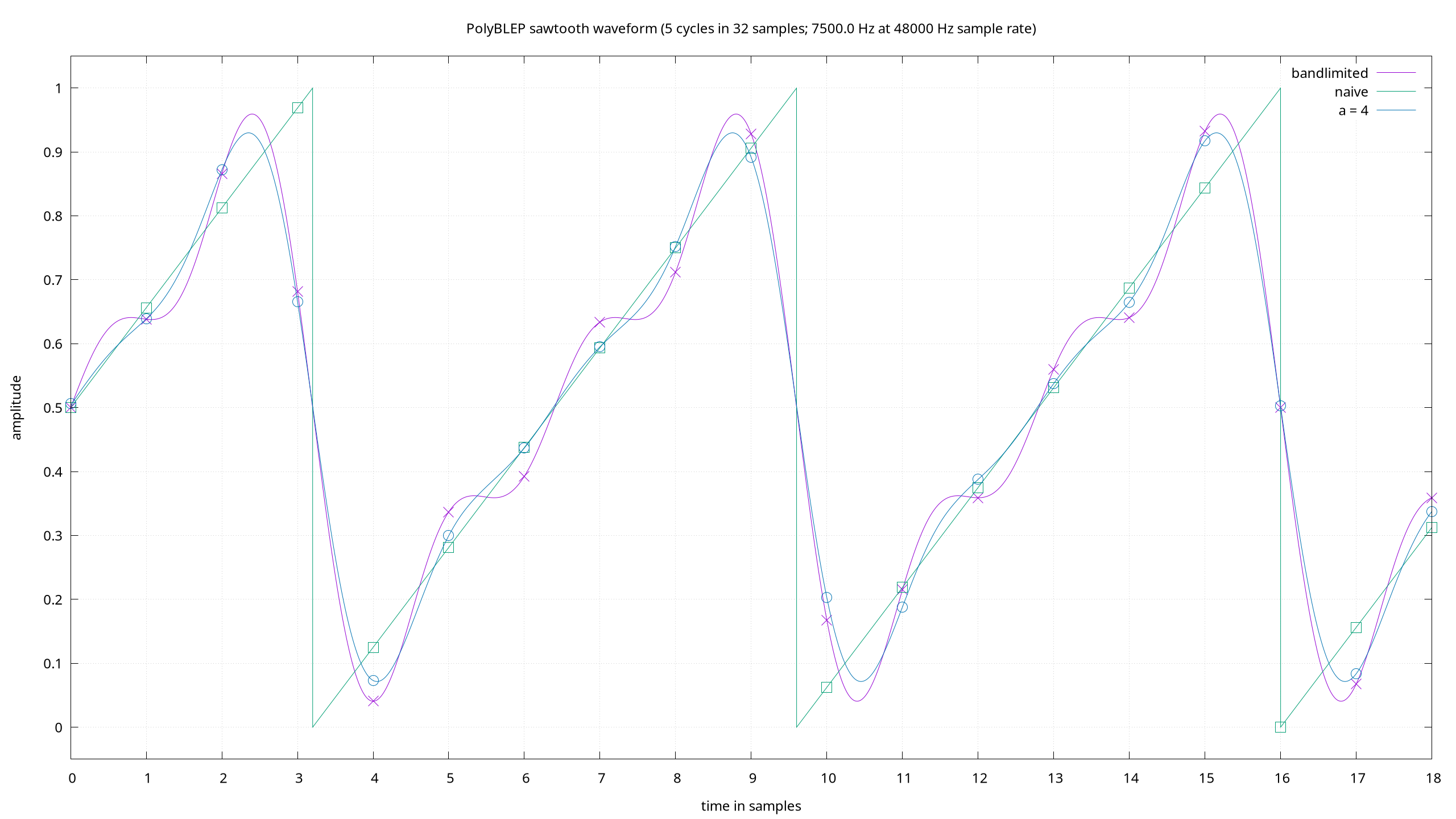
The aliasing comes from the sharp step discontinuities in the ideal sawtooth waveform. The strategy will be to replace the sharp steps with bandlimited steps.
A step function is the integral of the Dirac delta (aka impulse). A bandlimited Dirac impulse (with sample rate normalized to 1) is the sinc function .
Unfortunately the sinc function extends forever in both directions, so the next step is to window it with a function that is 0 everywhere outside a small support region.
I tried the window from a Lanczos filter which uses the central lobe of for small positive integer in the interval and 0 outside, but in my tests a raised cosine window worked much better: in the interval and 0 outside.
Unfortunately (again) these functions are hard to integrate. The strategy I adopted is to approximate the curve by a cubic spline through integer .
The cubic spline needs the value and slope at the end of each of the intervals . These can be calculated readily (differentiation is easier than integration):
Now the cubic spline for , letting be the fractional position, is defined by the matrix equation:
Piecewise polynomials are easy to integrate to piecewise polynomials : integrate each section symbolically, accumulating the value of as the constant of integration of (iteratively). Letting , the symbolic integration is simple:
where the precalculated is a constant vector of 5 real numbers, determined by the window size parameter . Then each cubic spline segment can be evaluated by a dot product with the same vector of powers of .
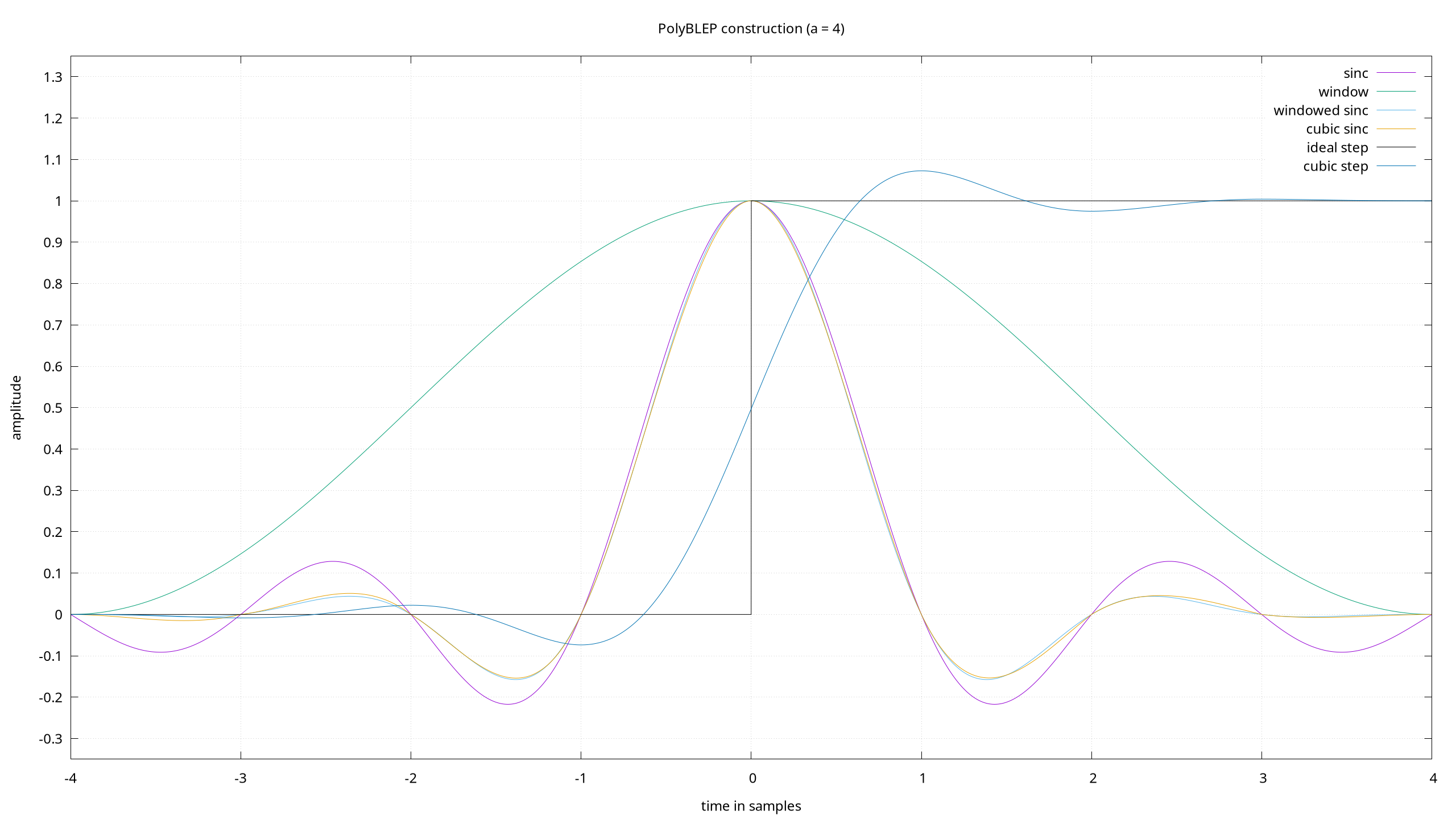
Now for a sawtooth waveform, we can sample the ramp part naively, but when we reach a step discontinuity we replace it with a bandlimited step by shifting the cubic spline (minus the ideal step) and adding it to the output waveform (scaled by the size of the input step, in this case -1, in other words subtraction).
We do this by calculating the subsample offset of the ideal discontinuity from the known frequency of the waveform. If the step occurs between samples and , with sawtooth values and , then is the slope of the ramp and at the discontinuity, which gives
Then calculate and compute the dot products with the precomputed .
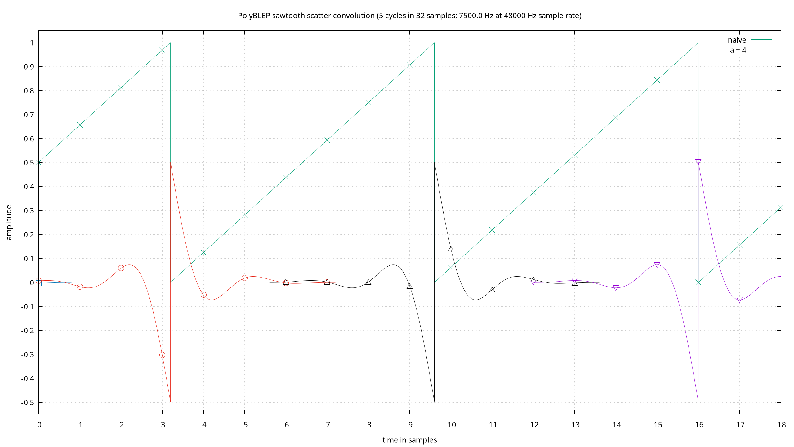
The output is accumulated into a rolling buffer of length : the regular values are added into and the PolyBLEPs are added into . This means the algorithm adds samples of latency.
The resulting waveform is smooth and close to the bandlimited curve (see first image above).
# 2 Spectrum
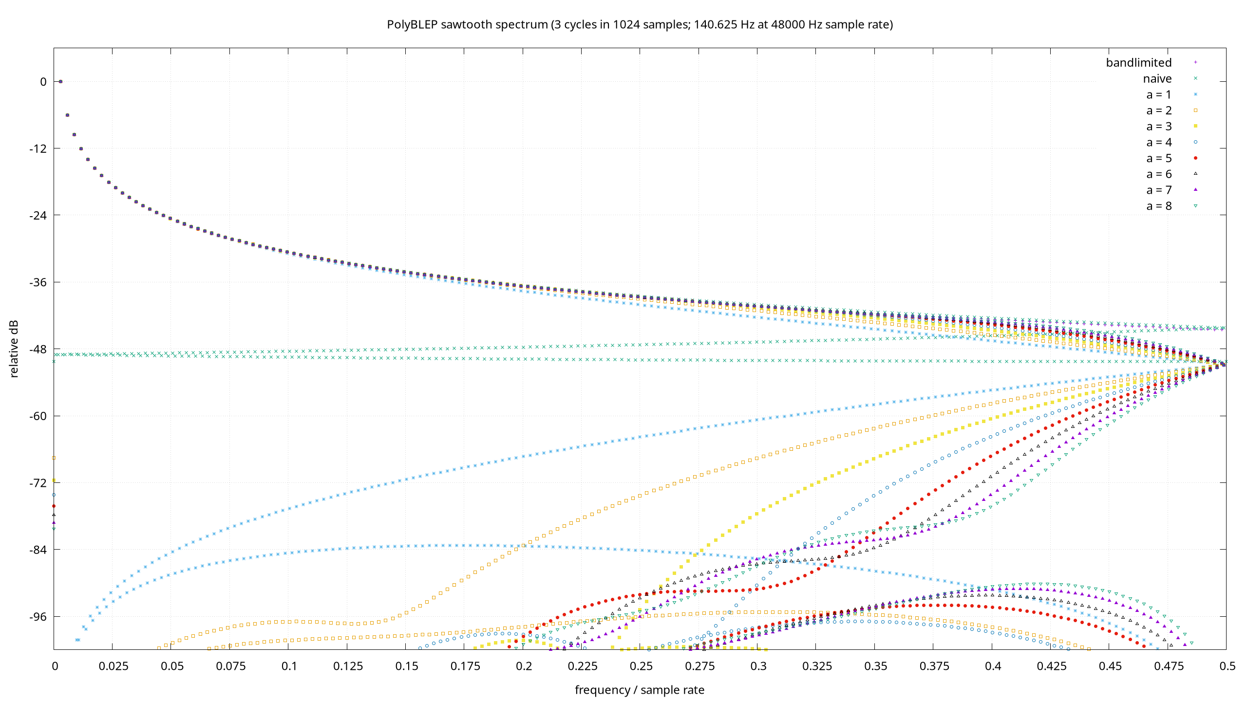
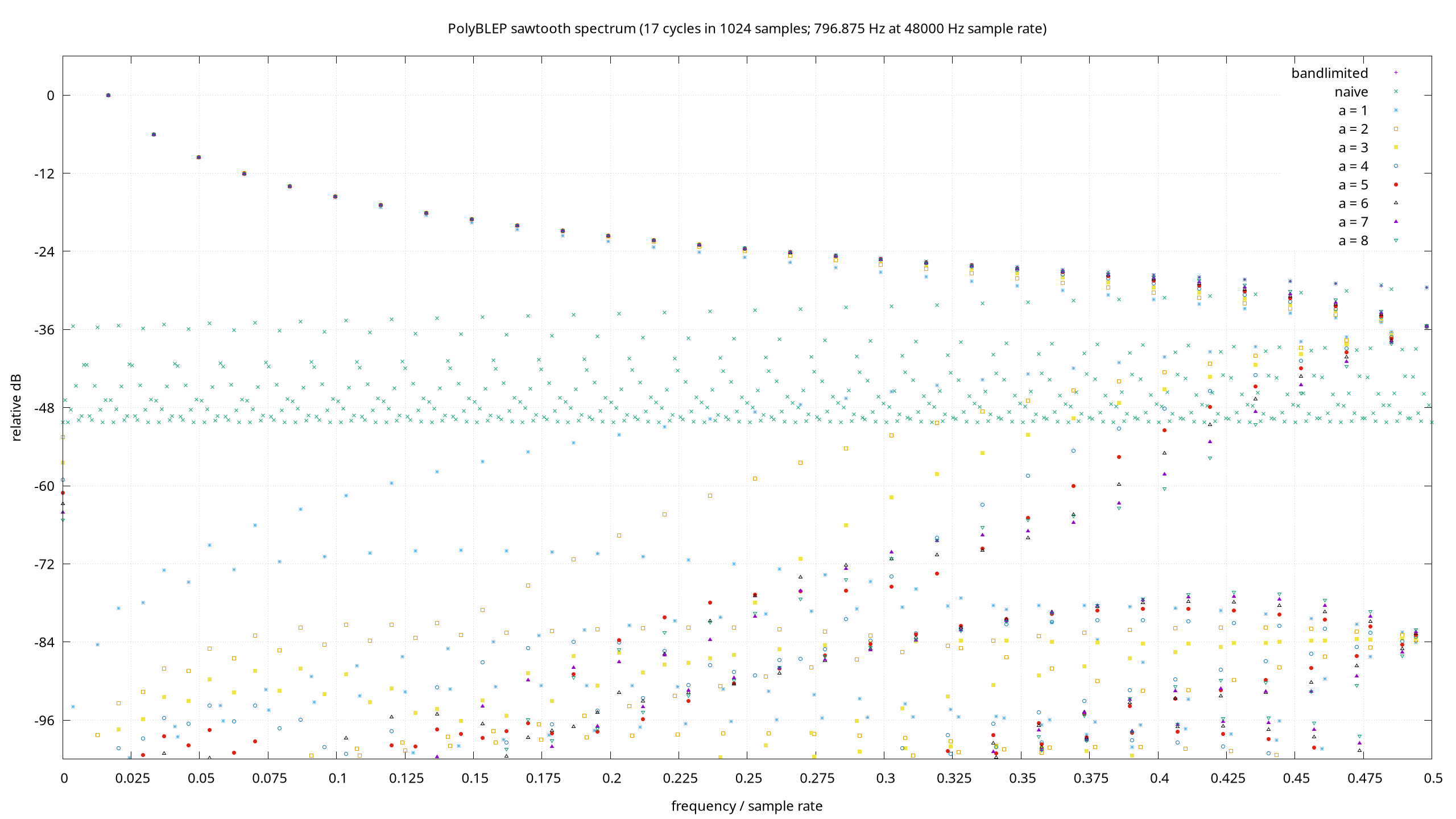
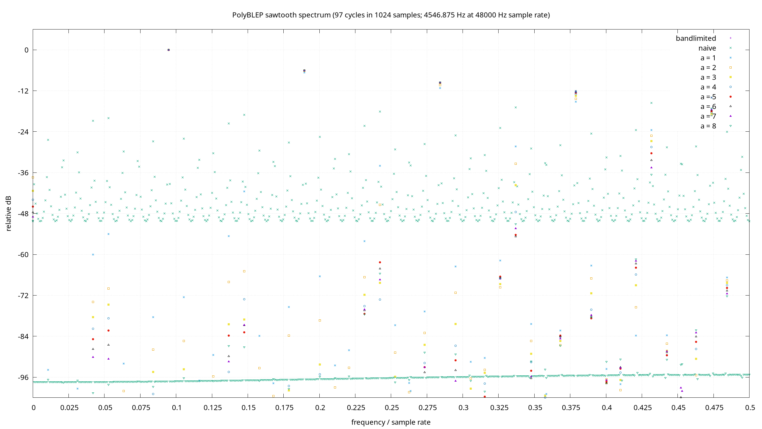
Plotting spectra shows that aliasing is reduced, especially at low frequencies, but high frequencies are reduced. Hence oversampling 2x may be needed for best results. Setting the parameter to , may be the best trade-off between quality and efficiency.
# 2.1 Low Frequency Saw
3 cycles in 1024 samples (140.625 Hz at 48000 Hz sample rate)
# 2.2 Mid Frequency Saw
17 cycles in 1024 samples (796.875 Hz at 48000 Hz sample rate)
# 2.3 High Frequency Saw
97 cycles in 1024 samples (4546.875 Hz at 48000 Hz sample rate)
# 3 Listen
In particular the high frequency naive saw sounds very bad.
# 3.1 Low Frequency Saw
3 cycles in 1024 samples (140.625 Hz at 48000 Hz sample rate)
- bandlimited
- naive
- a = 1
- a = 2
- a = 3
- a = 4
- a = 5
- a = 6
- a = 7
- a = 8
# 3.2 Mid Frequency Saw
17 cycles in 1024 samples (796.875 Hz at 48000 Hz sample rate)
- bandlimited
- naive
- a = 1
- a = 2
- a = 3
- a = 4
- a = 5
- a = 6
- a = 7
- a = 8
# 3.3 High Frequency Saw
97 cycles in 1024 samples (4546.875 Hz at 48000 Hz sample rate)
- bandlimited
- naive
- a = 1
- a = 2
- a = 3
- a = 4
- a = 5
- a = 6
- a = 7
- a = 8
# 4 Source Code
Licence: GNU AGPL, v3 only
- polyblep.c implementation in C
- polyblep.gnuplot plotting with gnuplot
- polyblep.sh driver script