# Hopfbrot
A 4D fractal formula related to the Mandelbulb.
History/credits:
- I saw this post on the Fediverse https://mastodon.gamedev.place/@idontlikenames/115605551174495073
- then I found the paper that defined(*) it: Oliver Knill, “Mandelbulb, Mandelbrot, Mandelring and Hopfbrot”, https://arxiv.org/abs/2305.17848
- @idontlikenames optimized some of the trigonometry
- I did polynomial conversion for power 2 (using Maxima)
- I implemented it in lycium et al’s FractalTracer, extending FT to support 4D dual numbers.
- I implemented it in Syntopia et al’s FragM using my fragm-examples dual number framework.
- I saw @idontlikenames article https://uehapetsijque.substack.com/p/the-hopfbrot.
- (*) I found bugman’s original forum post from 2009: https://www.fractalforums.com/theory/3d-mandelbrot-formula-based-on-the-hopf-map/ (archived copy, archived copy)
# 1 Formula
# 1.1 Trigonometric
The Hopfbrot formula is specified using hyperspherical trigonometry with vector power similar to the Mandelbulb. Pseudo-code:
formula(z, c):

  z = hopf(z, power) + c;

hopf(z, power):

  r = length(z);
  t = atan2(length(z.zw), length(z.xy));
  u = atan2(z.y, z.x);
  v = atan2(z.w, z.z);

  r = pow(r, power)
  t = t * power;
  u = u * power;
  v = v * power

  return
    { r * cos(t) * cos(u)
    , r * cos(t) * sin(u)
    , r * sin(t) * cos(v)
    , r * sin(t) * sin(v)
    };
Image rendering can be done via ray marching with automatic differentiation for distance estimates, for example code see github.com/lycium/FractalTracer.
# 1.2 Polynomial (Power 2)
I used Maxima computer algebra system to
work out the maths for power 2 hopf(). A similar approach
should work for other integer powers.
The key identities are:
cos(2 * atan2(y, x)) = (x^2 - y^2) / (x^2 + y^2)
sin(2 * atan2(y, x)) = 2 * x * y / (x^2 + y^2)
giving pseudo-code:
hopfPoly2(p):

  x2 = p.x * p.x;
  y2 = p.y * p.y;
  z2 = p.z * p.z;
  w2 = p.w * p.w;
  x2y2 = x2 + y2;
  z2w2 = z2 + w2;

  cos2u = (x2 - y2) / x2y2;
  sin2u = 2 * x * y / x2y2;
  cos2v = (z2 - w2) / z2w2;
  sin2v = 2 * z * w / z2w2;
  r2cos2t = x2y2 - z2w2;
  r2sin2t = 2 * sqrt(x2y2 * z2w2);

  return
    { r2cos2t * cos2u
    , r2cos2t * sin2u
    , r2sin2t * cos2v
    , r2sin2t * sin2v
    };
The hopfPoly2(z) is about 2x faster than the
trigonometric hopf(z, 2), when tested on CPU with
FractalTracer.
# 2 Perturbation
Fractal iterations can be perturbed for efficient deep zooming,
# 2.1 Trigonometric Perturbation
TODO. Might be more efficient than polynomial due to the latter’s length.
# 2.2 Polynomial Perturbation
Here is the power 2 polynomial version perturbed using the Maxima computer algebra system:
display2d : false$

/* the Hopf power 2 polynomial implementation */

s(x,y,z,w) := (x^2 + y^2 - z^2 - w^2) * (x^2 - y^2) / (x^2 + y^2)$
t(x,y,z,w) := (x^2 + y^2 - z^2 - w^2) * (2 * x * y) / (x^2 + y^2)$
u(x,y,z,w) := 2 * sqrt((x^2 + y^2) * (z^2 + w^2)) * (z^2 - w^2) / (z^2 + w^2)$
v(x,y,z,w) := 2 * sqrt((x^2 + y^2) * (z^2 + w^2)) * (2 * z * w) / (z^2 + w^2)$

/* Maxima can perturb simple functions */

p(f) := factor(expand(f(X+x,Y+y,Z+z,W+w) - f(X,Y,Z,W)))$

p(s);

p(t);

/* make it easier by putting everything inside one sqrt */

uu(x,y,z,w) := sqrt(4 * (x^2 + y^2) * (z^2 + w^2) * (z^2 - w^2)^2 / (z^2 + w^2)^2)$

vv(x,y,z,w) := sqrt(4 * (x^2 + y^2) * (z^2 + w^2) * (2 * z * w)^2 / (z^2 + w^2)^2)$

/* perturb difference of sqrt by multiplying top and bottom by sum of sqrt */
/* the top becomes a difference of squares which can be simplified */

pp(f) :=
factor(
expand(f(X+x,Y+y,Z+z,W+w)^2 - f(X,Y,Z,W)^2) /
      (f(X+x,Y+y,Z+z,W+w)   + f(X,Y,Z,W)  )
)$

pp(uu);

pp(vv);

/* small issue: sqrt(a^2) becomes abs(a) instead of a, fix in post? */
Output not shown due to length.
Not yet tested. I used Maxima 5.47.0 on Termux.
# 3 Linear Approximation
Should be possible, with 4x4 matrices for coefficients of xyzw and abcd.
The hard part will probably be calculating the validity radii.
The singular values of the single step Jacobian (w.r.t XYZW) are surprisingly simple:
sqrt(16*(X^2+Y^2))sqrt(4*(Z^2+W^2-X^2-Y^2)^2/(X^2+X^2))sqrt(4*(X^2+Y^2+Z^2+W^2))(with multiplicity 2)
Calculated with Maxima:
S : s(X,Y,Z,W)$
T : t(X,Y,Z,W)$
U : u(X,Y,Z,W)$
V : v(X,Y,Z,W)$

J : factor(expand(matrix(
[diff(S, X), diff(S, Y), diff(S, Z), diff(S, W)],
[diff(T, X), diff(T, Y), diff(T, Z), diff(T, W)],
[diff(U, X), diff(U, Y), diff(U, Z), diff(U, W)],
[diff(V, X), diff(V, Y), diff(V, Z), diff(V, W)])));

e : (eigenvalues(J . transpose(J)));
# 4 Animations
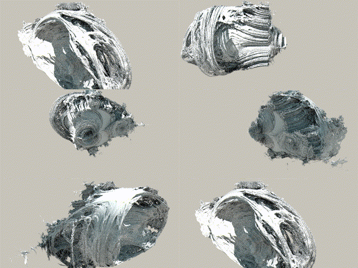
The whole set looks like it has some familiar cross-sections:
The main mini on the antenna looks like a 3D Burning Ship:
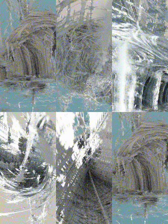
Both animations rendered with FractalTracer using dual numbers with the 4th derivative component set to 0, in the w=0 3D slice. Using full 4D derivatives makes the set blobby.