# Lambdabulb
A 3D fractal formula related to the Mandelbulb.
History/credits:
- Fractal Chats Discord discussion August 2024
- original definition at fractalforums.com/mandelbulb-renderings/lambdabulb,
- modified by machina-infinitum
- fragmentarium version assisted by dark-beam
- translated to lycium et al’s FractalTracer by bezo97
- polynomial optimization by me
# 1 Formula
\[ z \to c (z - z^p)\]
# 1.1 Trigonometric
The Lambdabulb formula is specified using spherical trigonmetry with a “triplex” vector multiplication and power similar to the Mandelbulb. Pseudo-code:
formula(z, c):

  z = triplexMult(c, z - triplexPow(z, power, phase));

triplexPow(z, power, phase):

  r = length(z);
  theta = atan2(z.y, z.x);
  phi = acos(z.z / r);

  r = pow(r, power)
  theta = theta * power;
  phi = phi * power + phase;

  return
    { r * sin(phi) * cos(theta)
    , r * sin(phi) * sin(theta)
    , r * cos(phi)
    };

triplexMul(u, v):

  ru = length(u);
  rv = length(v);
  a = 1 - (u.z * v.z) / (ru * rv);
  return
   { a * (u.x * v.x - u.y * v.y)
   , a * (v.x * u.y + u.x * v.y)
   , rv * u.z + ru * v.z
   };
Image rendering can be done via ray marching with automatic differentiation for distance estimates, for example code see github.com/lycium/FractalTracer.
# 1.2 Polynomial (Power 4)
Profiling with valgrind --tool=cachegrind showed that
50% of the program runtime was in libm for the trigonmetry and powers.
Similar to Chebyshev polynomials,
trig(f(inverse trig)) can often be replaced by algebra,
which is usually less computationally expensive
and sometimes more accurate.
I used wxMaxima computer algebra system to work out the maths for power 4 triplexPow. A similar approach should work for other integer powers.
(%i1)	power : 4;
(%o1)	4
(%i2)	factor(trigexpand(cos(power*atan2(y,x))));
(%o2)	((y^2-2*x*y-x^2)*(y^2+2*x*y-x^2))/(y^2+x^2)^2
(%i3)	factor(trigexpand(sin(power*atan2(y,x))));
(%o3)	-(4*x*y*(y-x)*(y+x))/(y^2+x^2)^2
(%i4)	at(factor(expand(trigexpand(factor(trigexpand(cos(phase + power * acos(z / sqrt(x^2+y^2+z^2)))))))), [cos(phase) = c, sin(phase) = s]);
(%o4)	(c*z^4-4*s*sqrt(y^2+x^2)*z^3-6*c*y^2*z^2-6*c*x^2*z^2+4*s*y^2*sqrt(y^2+x^2)*z+4*s*x^2*sqrt(y^2+x^2)*z+c*y^4+2*c*x^2*y^2+c*x^4)/(z^2+y^2+x^2)^2
(%i5)	at(factor(expand(trigexpand(factor(trigexpand(sin(phase + power * acos(z / sqrt(x^2+y^2+z^2)))))))), [cos(phase) = c, sin(phase) = s]);
(%o5)	(s*z^4+4*c*sqrt(y^2+x^2)*z^3-6*s*y^2*z^2-6*s*x^2*z^2-4*c*y^2*sqrt(y^2+x^2)*z-4*c*x^2*sqrt(y^2+x^2)*z+s*y^4+2*s*x^2*y^2+s*x^4)/(z^2+y^2+x^2)^2
With some manual common subexpression elimination,
and noting that dividing cos_phi and sin_phi by \(r^4\) is unnecessary
as the end result is multiplied by \(r^4\),
this translates into pseudo-code like so:
triplexPow4(z, cos_phase, sin_phase):

  x2 = z.x * z.x;
  y2 = z.y * z.y;
  z2 = z.z * z.z;
  xy2 = 2 * z.x * z.y;
  y2mx2 = y2 - x2;
  y2px2 = y2 + x2;
  y2px22 = y2px2 * y2px2;

  cos_theta = (y2mx2 - xy2) * (y2mx2 + xy2) / y2px22;
  sin_theta = -2 * xy2 * y2mx2 / y2px22;

  z22 = z2 * z2;
  a = z22 + y2px22 - 6 * y2px2 * z2;
  b = sqrt(y2px2) * z.z * (z2 - y2px2);
  cos_phi = cos_phase * a - 4 * sin_phase * b;
  sin_phi = sin_phase * a + 4 * cos_phase * b;

  return
    { sin_phi * cos_theta,
    , sin_phi * sin_theta,
    , cos_phi
    };
# 2 Benchmarks
FractalTracer compiled with g++ 12 on AMD Ryzen 2700X CPU (16 threads) running Debian Bookworm, at 1280x720 resolution. Lower timings are better.
- trigonometric, double precision, double epsilon: 126 seconds per pass
- trigonometric, double precision, single epsilon: 58 seconds per pass
- trigonometric, single precision, double epsilon: 73 seconds per pass
- trigonometric, single precision, single epsilon: 36 seconds per pass
- polynomial, double precision, double epsilon: 78 seconds per pass
- polynomial, double precision, single epsilon: 40 seocnds per pass
- polynomial, single precision, double epsilon: 42 seconds per pass
- polynomial, single precision, single epsilon: 22 seconds per pass
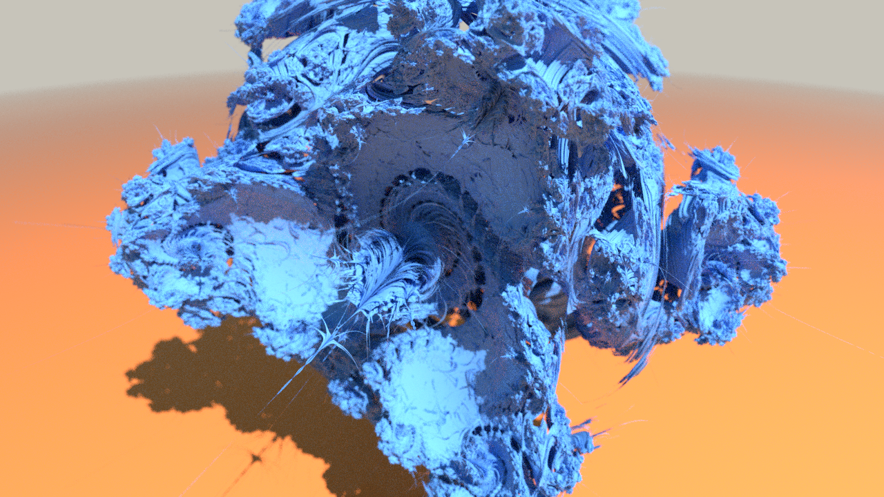
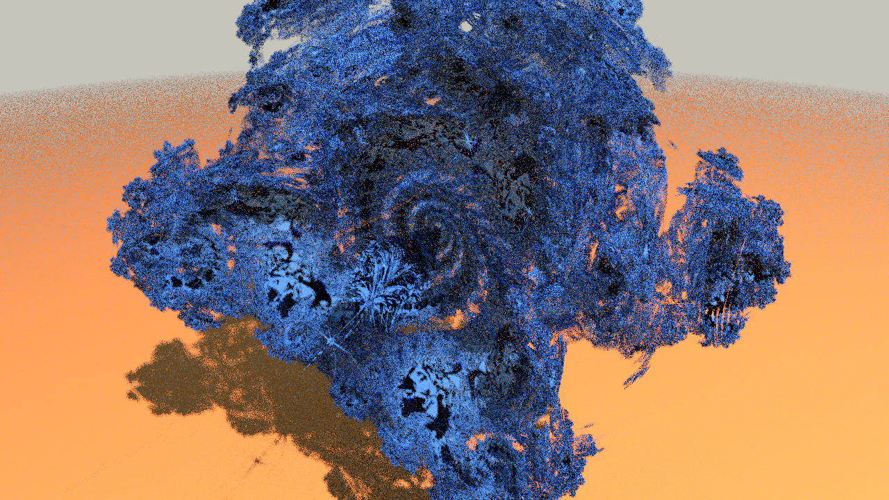
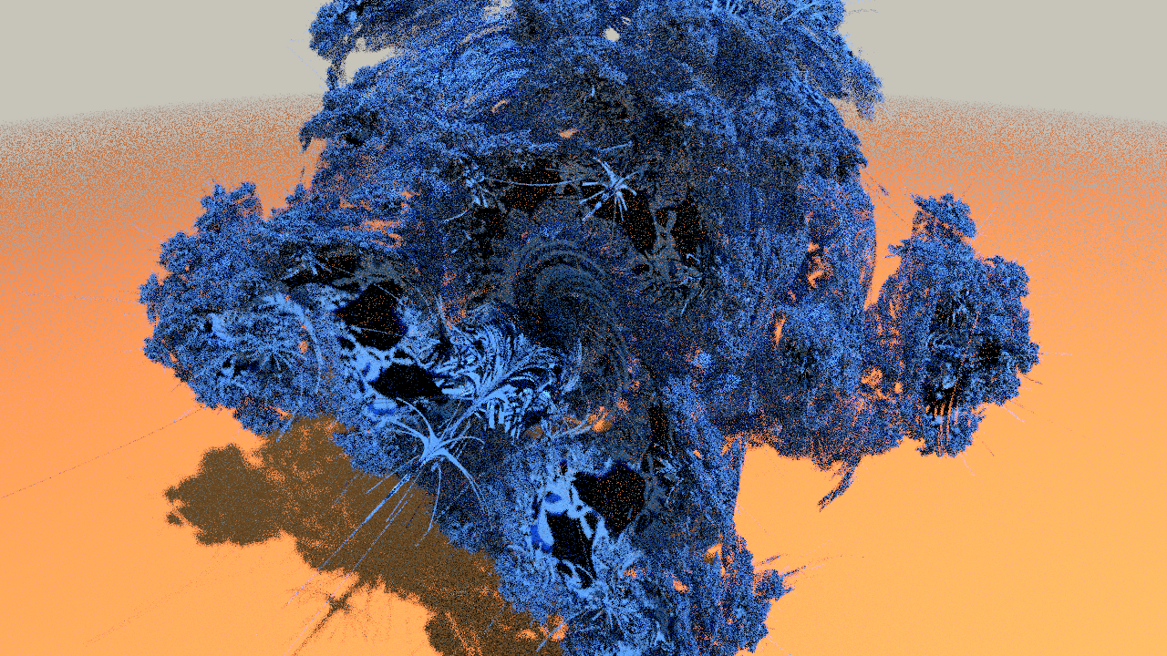
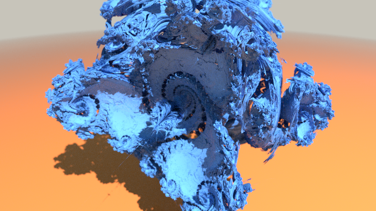
# 3 Images
Comparison of trigonometric (4 samples per pixel) vs polynomial (32 samples per pixel), double vs single floating point precision, double vs single tuned ray marching epsilons.
Using single-tuned epsilons (which are larger) has the effect of thickening the fractal shape.
Polynomial seems improved over trigonometric, the fractal is much more solid. Not sure whether there is a bug somewhere or if it’s just numerical precision issues.
Note the different appearance near the horizon of the penultimate polynomial-single-double image, this is probably due to self-intersections caused by to too-low epsilons for the precision.
Parameters:
power = 4
phase = 1.815142
c = { 1.035, -0.317, 0.013 }
The fixed c makes it a “Juliabulb” variant.
- trigonometric, double precision, double epsilon

- trigonometric, double precision, single epsilon

- trigonometric, single precision, double epsilon
- trigonometric, single precision, single epsilon
- polynomial, double precision, double epsilon
- polynomial, double precision, single epsilon
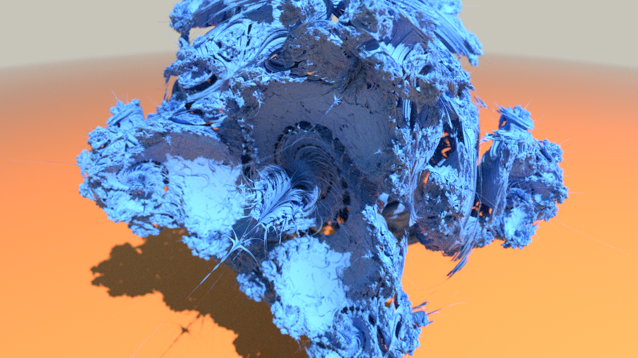
- polynomial, single precision, double epsilon

- polynomial, single precision, single epsilon