# Nebuloculars
Work in progress, binoculars for the nebulabrot.
# 1 Problem
It is hard to zoom in the nebulabrot, because it is hard to find c values that iterate from z = 0 to z near a small target.
# 2 Region Selection
# 2.1 Homotopy
Construct a differential equation to find two roots of fp+1(c, 0) = t given one root of fp(c, 0) = t.
Doesn’t really work, there are too many roots (O(2p)), and most of them hit near the target only once before escaping.
Only suitable for small p (10s), but for deep zooms p needs to be much higher (100ks).
Microblog thread: https://post.lurk.org/@mathr/116201222838737968
Reference for the method for Mandelbrot set roots:
“A comparison of solution methods for Mandelbrot-like polynomials” Eunice Y. S. Chan, MSc thesis, The University of Western Ontario https://ir.lib.uwo.ca/etd/4028/ https://uwo.scholaris.ca/server/api/core/bitstreams/2cf58b26-c757-48e1-833c-bda6c70a1e18/content
# 2.2 Cell Mapping
Use a cell mapping approach to prove that certain regions cannot hit the target more than once.
Uses vast amounts of memory, so parallelism opportunities are limited.
Doesn’t really work, the remaining unrejected region is too large so histogram hit rate is still tiny.
Microblog thread: https://post.lurk.org/@mathr/116218542001920018
# 2.3 Distance Estimate
Estimate how far c would have to be perturbed for the orbit to hit the target (iterating z from 0):
Dc = min |(z - t) / (dz/dc)|
Estimate how far z is from the target to see if it hits the target more than once (iterating z from the target):
Dz = min |(z - t)|
Keep boxes that are close enough, with Dc and Dz less than thresholds proportional to box size until box gets smaller than target view size:
threshold = max(box size, view radius) × 32
Refine by subdivision.
Uses small constant memory, streaming from/to files.
Optionally: reject boxes that are entirely interior (using interior distance estimate). Time is eventually completely dominated by interior distance calculations.
Problem: this method is probably not unbiased…
# 2.4 Importance Sampling
The previous algorithm is biased, because some rejected regions might actually contain points that hit the target.
An alternative algorithm uses importance sampling,
which distributes probability over the [-2,2]2 square
such that integrated over
any nonempty subregion it is nowhere 0, with samples weighted
proportionally to area/probability
(weight proportional to area to simulate uniform sampling).
AFAIK this is (asymptotically?) unbiased no matter the precise details of the proposed probability distribution (just need non-zero everyhere). The closer the computed proposed distribution is to the actual distribution (which is unknown) the better the estimate will be (lower variance).
Region subdivision is guided by seeing if any sample orbit (of max 1k trials or so) within a region has at least two hits to the target viewport. Target viewport starts at the full set and zooms in to the desired view during subdivision.
Histogram accumulation gives regions probability proportional to 1/area and weight proportional to area/probability.
# 3 Histogram Accumulation
Histogram has N layers at 2x iteration count boundaries.
Either clamp betwen lowest highest layer when plotting, or drop out of range (too low/high iteration count).
# 3.1 Analysis
Pick a random c in one of the boxes.
Iterate z from 0.
If |z| reaches a new minimum at iteration p, check for interior:
-
Newton’s method to solve fcp(z0) = z0
-
if |dfcp(z0)/dz0| <= 1 then interior to component of period p, stop
If z is in the view near the target
-
increment hit counter
-
set hit z to z
If |z| escaped, proceed to plot phase.
# 3.2 Plot
If |z| escaped and hit counter = 1, plot hit z
If |z| escaped and hit counter > 1, iterate z from 0 until escape iteration count plotting all z that hit the view. No need for escape or interior tests.
# 3.3 Anti-Aliasing
# 3.3.1 Deterministic
To plot: find floating point pixel coordinates corresponding to z, log2(escaped iteration count). Compute integer coordinates of 8 neighbouring histogram buckets and use the fractional part of the coordinates to weight them. For each of the 8 buckets, check that integer coordinates are in view, atomic add to histogram layer k coordinates i j.
Problem: 8 atomic adds are excessive.
# 3.3.2 Stochastic
To plot: find floating point pixel coordinates corresponding to z, log2(escaped iteration count).
Add a pseudo random offset in [0,1) to i j k for dithering / anti-aliasing.
Convert to integer coordinates.
Check that integer coordinates are in view.
Atomic add to histogram layer k coordinates i j.
# 3.4 Mipmaps
If the histogram is too big for the number of samples, there are gaps between speckles and tonemapping doesn’t work properly.
# 3.4.1 Downscale
Accumulate into one large histogram. When tonemapping, downscale histogram by summing buckets.
Problem: no antialiasing in smaller histograms.
# 3.4.2 Upfront
Accumulate simultaneously into multiple mipmap levels up to a maximum size, inspect images after tonemapping each to see which size looks best.
Problem: multiplies the number of atomic adds by the number of layers.
# 3.4.3 Progressive
Start with a small image (e.g. 1x1).
Once enough samples per pixel have been accumulated (e.g. 256), upscale the histogram, ensuring that total contribution remains the same.
Continue accumulating until histogram is as large as desired. With 2x scaling, each next image takes 4x longer.
Problem: it looks bad (multi-scale pixelation / blur).
# 4 Tone Mapping
Multiply each log2(iteration count) layer by an RGB colour.
Sum all layers.
Transform to log(1 + count)
Divide by maximum, square root (for approximate sRGB gamma),
multiply by 255 (for 8 bit output),
adding a pseudorandom number in range [0,1) for dithering
to reduce banding.
Output as PPM piped through NetPBM pnmtopng to a PNG file.
# 5 Examples
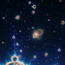
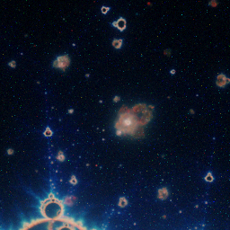
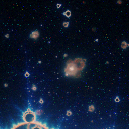
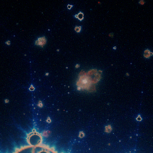
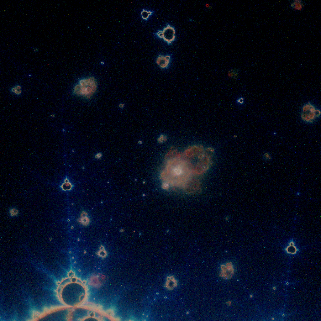
# 5.1 Deep Field
Reconstruction of tavis’ Deep Field Nebulabrot location:
z-plane coordinates:
x0: 0.56208345369277852973
y0: 0.00000016540178571429
r0: 1e-8
iteration thresholds:
B:  60000 -   180000
G: 180000 -   600000
R: 600000 - 60000000
orbit density:
~460 orbits plotted (> 0 hits) per pixel
# 5.1.1 Results
Preprocessing gives 2065 cells in ~10 minutes.
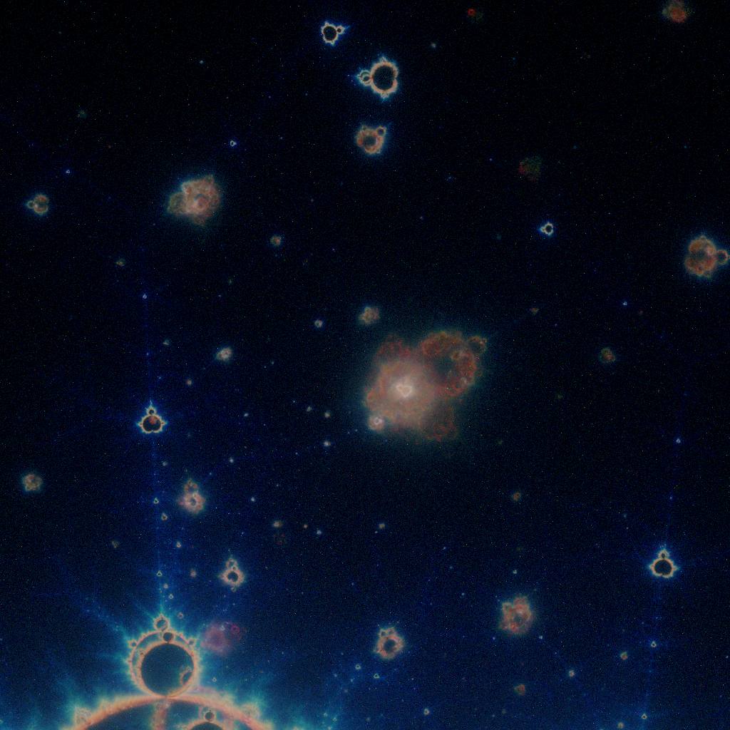
Images after about 42mins (left) and 85mins (right) histogram computation wall-clock on laptop (decaf) with 16 threads.
# 5.1.1.1 64x64


# 5.1.1.2 128x128

# 5.1.1.3 256x256
# 5.1.1.4 512x512

# 5.1.1.5 1024x1024
# 5.1.2 Convergence
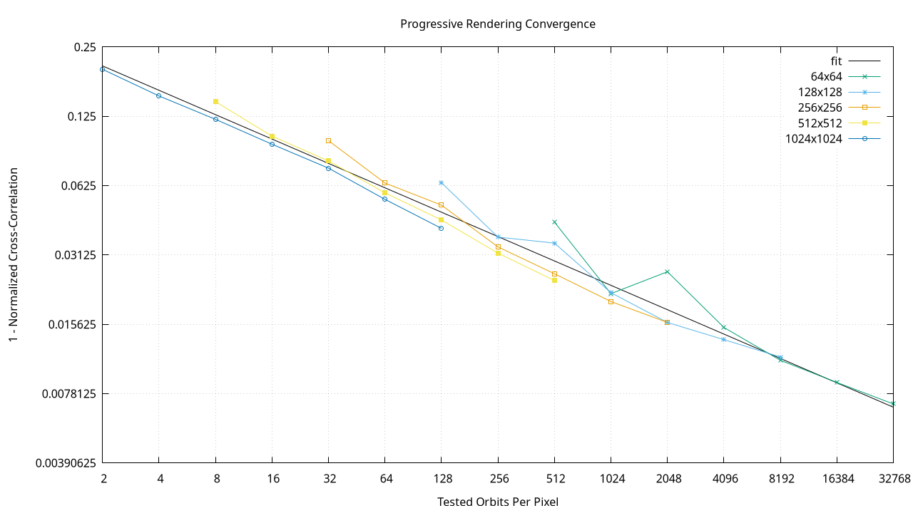
Use ImageMagick compare -metric NCC between images after doubling the number of tested orbits. Plot 1-ncc against orbits per pixel on a log-log scale, with line fitted with gnuplot.
Fitted line has slope approximately -sqrt(1/8). This means halving 1-ncc requires increasing tested orbits per pixel by a factor of approximately 7.1.
The noise floor measured for 8-bit images is 1-ncc = 3.4×10⁻⁵. Full convergence down to the noise floor may take estimated 1027 orbits per pixel.
# 6 Implementation
# 6.1 Quick Start
git clone https://code.mathr.co.uk/nebuloculars.git
cd nebuloculars
mkdir out
cd out
../nebuloculars.sh
# 6.2 Components
Several programs make up the system:
-
neb-boxes-to-cells: convert boxes to cells
-
neb-cell-mapping: refine cells using cell mapping
-
neb-density: refine boxes using sampled hits
-
neb-distance-estimate: refine cells using distance estimates
-
neb-histogram: sample points from cells and accumulate hits. initial invocation creates histogram testing a million orbits, subsequent passes double the number of tested orbits.
-
neb-histogram-merge: merge histograms (e.g. after parallel processing on multiple machines)
-
neb-image: visualize cells as a 2D image
-
neb-noise-floor: generate image pairs suitable for measuring noise floor
-
neb-progress: process log data for curve fitting
-
neb-progress.gnuplot: graph log data
-
neb-split: split cells into several parts (e.g. before parallel processing on multiple machines; afterwards combine with cat)
-
neb-tonemap: visualize histogram as a 2D image
-
nebuloculars.sh: script to render image
All are subject to change with various hard-coded configurations. Various branches in the git repository have different features.
# 7 Related Work
- Tavis’ “Deep Field Nebulabrot”
- Fractal Universe’s “James-Webb for Buddhabrot”