mathr / blog / #

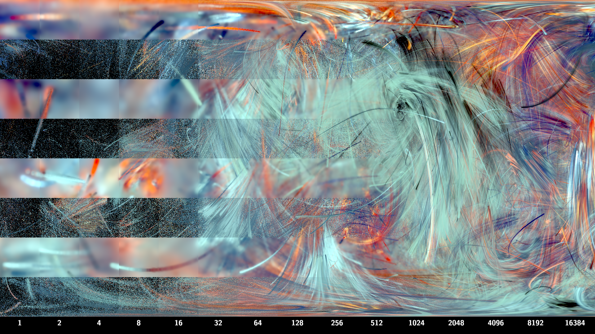
Vertical slices (constant x) have the same number of samples per pixel. number of samples doubles each slice, from 1 at the left to 16384 at the right. Horizontal slices (constant y) have density estimation on or off. The top slice has density estimation on, the bottom slice has density estimation off. Below the bottom slice are numbers indicating samples per pixel Quality is low at the left and high at the right. With density estimation, the left image is blurry but about the same brightness as the right hand side. Without density estimation, the left image is sparse and noisy, and much darker due to the black background. Towards the right hand side both methods converge to the same image.

Fractal flames are generated by applying the chaos game technique to a weighted directed graph iterated function system with non-linear functions. Essentially what this means is, you start from a random point, and repeatedly pick a random transformation from the system and apply it to the point - plotting all the points into an histogram accumulation buffer, which ends up as a high dynamic range image that is compressed for display using a saturation-preserving logarithm technique.

The main problem with the chaos game is that you need to plot a lot of points, otherwise the image is noisy. So to get acceptable images with fewer numbers of points, an adaptive blur algorithm is used to smooth out the sparse areas, keeping the dense areas sharp:

Adaptive filtering for progressive monte carlo image rendering

by Frank Suykens , Yves D. Willems

The 8-th International Conference in Central Europe on Computer Graphics, Visualization and Interactive Digital Media 2000 (WSCG' 2000), February 2000. Held in Plzen, Czech Republic

Abstract

Image filtering is often applied as a post-process to Monte Carlo generated pictures, in order to reduce noise. In this paper we present an algorithm based on density estimation techniques that applies an energy preserving adaptive kernel filter to individual samples during image rendering. The used kernel widths diminish as the number of samples goes up, ensuring a reasonable noise versus bias trade-off at any time. This results in a progressive algorithm, that still converges asymptotically to a correct solution. Results show that general noise as well as spike noise can effectively be reduced. Many interesting extensions are possible, making this a very promising technique for Monte Carlo image synthesis.

The problem with this density estimation algorithm as presented in the paper is that it is very expensive: asymptotically it's about \(O(d^4)\) where \(d\) is the side length of the image in pixels. It's totally infeasible for all but the tiniest of images. But I did some thinking and figured out how to make it \(O(d^2)\), which at a constant cost per pixel is the best it is possible to do.

So, starting with the high dynamic range accumulation buffer, I compute a histogram of the alpha channel with log-spaced buckets. As I am using ulong (uint64_t) for each channel, a cheap way to do this is the clz() function, which counts leading zeros. The result will be between 0 and 64 inclusive. Now we have a count of how many pixels are in each of the 65 buckets.

For each non-empty bucket (that doesn't correspond to 0), threshold the HDR accumulation buffer to keep only the pixels that fall within the bucket, setting all the rest to 0. Then blur this thresholded image with radius inversely proportional to \(\sqrt{\text{bucket value}}\) (so low density is blurred a lot, highest density is not blurred at all). And then sum all the blurred copies into a new high dynamic range image, before doing the log scaling, auto-white-balance, gamma correction, etc as normal.

The key to making it fast is making the blur fast. The first observation is that Gaussian blur is separable: you can do a 2D blur by blurring first horizontally and then vertically (or vice versa), independently. The second observation is that repeated box filters tend to Gaussian via the central limit theorem. And the third important observation is that wide box filters can be computed just as cheaply as narrow box filters by using a recursive formulation:

for (uint x = 0; x < width; ++x)
{
  acc -= src[x - kernel_width];
  acc += src[x];
  dst[x] = acc / kernel_width;
}

There is some subtlety around initializing the boundary conditions (whether to clamp or wrap or do something else), and to avoid shifting the image I alternate between left-to-right and right-to-left passes. A total of 8 passes (4 in each dimension, of which 2 in each direction) does the trick. There are at most 64 copies to blur, but in practice the number of non-empty buckets is much less (around 12-16 in my tests).

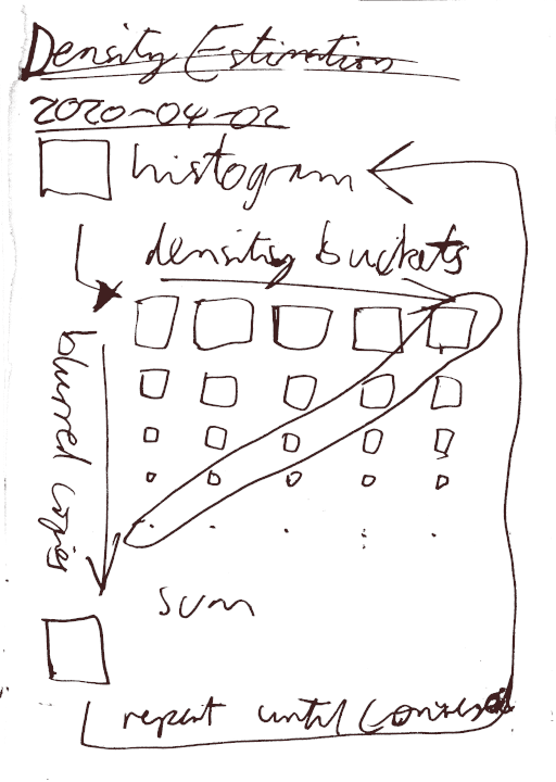
As a bonus, here's the page from my notebook where I first developed this fast technique:

Thanks to lycium for pointing out to me the second and third observations about box filters.

EDIT: I benchmarked it a bit more. At large image sizes (~8k^2) with extra band density (needed to avoid posterization artifacts from filter size quantization), it's about 40x slower (2mins) than Fractorium (5secs). If the sample/pixel count not ridiculously small they are indistinguishable (maybe mine is a very tiny bit smoother in less dense areas); for ridiculously small sample counts mine is very blurry and Fractorium's is very noisy, but 2mins iteration and 5secs filter definitely beats 5secs iteration and 2mins filter in terms of visual quality any way you do it. So I guess it's "nice idea in theory, but in practice...".