Counting artificial neural networks
On math.stackexchange.com, user Vincent asked a question that caught my attention:
I wanted to test different Networks with the same number of parameters but with different depths and widths.
A good introduction is in
Neural Networks and Deep Learning,
but in short: a neural network is essentially a chain of matrix
multiplies with non-linear "activation functions" in between (which
don't change the length of the vector of data passing through).
Matrices are 2D grids of numbers. Matrices can only be multiplied
together if the number of columns of the first matrix is equal to the
number of rows of the second matrix, so you can express the "shape" of
the neural network by a vector of positive integers, where each pair of
neighbouring values corresponds to the dimensions of one of the
matrices. The total number of parameters of the neural network is the
sum of the products of each such pair, for example the shape [3,7,5,1]
has size 3×7 + 7×5 + 5×1 = 61, which in the programming language Haskell
can be written size = sum (zipWith (*) shape (tail shape)).
The question is essentially asking that, given the size, to construct some different shapes with that size, in particular shapes of different length (corresponding to different depths of network). But to see how the problem looks, I decided to generate all possible shapes for a given size, starting with some hopelessly naive Haskell code:
import Control.Monad (replicateM)
shapes p =
  [ s
  | m <- [0..p]
  , s <- replicateM (m + 2) [1..p]
  , p == sum (zipWith (*) s (tail s))
  ]
main = mapM_ (print . length . shapes) [1..]
This code does "work", but as soon as the size p gets large, it takes forever and runs out of memory. On my desktop which has 32GB of RAM, I can only print 8 terms before OOM, which takes about 6m37s. These terms are:
1, 3, 5, 10, 14, 27, 37, 65
So a smarter solution is needed. I decided to implement it in C, because it's easier to do mutation there than Haskell. The core of the algorithm is the same as the Haskell above, but with one important addition: pruning. If the sum exceeds p before the end of the shape vector is reached, it doesn't make any difference what the suffix is: because all the dimensions are positive, the sum can never get smaller again.
I loop through depths (length of shape) until the maximum depth, as in the Haskell, and for each depth I start with a shape of all 1s, with last element 0 as an exception (it will be incremented before use). Each iteration of a loop, add 1 to the last element of the shape, if it gets bigger than the target p I set it back to 1 and propagate a carry 1 to the previous element (and so on). If the carry propagates beyond the first element, that means we've searched the whole shape space and we exit the loop.
Pruning is implemented by accumulating the sum from the left. If the sum of the first P products exceed the target, then set the whole shape vector starting from the (P+1)th index to the target, so at the next iteration of the loop, the last one is incremented and they all wrap around to 1, with the Pth item eventually incremented by 1. If the sum of all the products is equal to P, increment a counter (which is output at the end). I verified that the first 8 terms output with pruning matched the 8 terms output by my Haskell (without pruning), which is not a rigourous proof that the pruning is valid, but does increase confidence somewhat.
Because the C algorithm uses much less space than the Haskell (I do not know why that is so bad), and is much more efficient (due to pruning), it's possible to calculate many more terms. So much so that issues of numeric overflow come into play. Using unsigned 8 bit types for numbers allows only 11 terms to be calculated, because the counter overflows (term 12 is 384 > 2^8-1 = 255). The terms increase rapidly, so I decided to use 64 bits unsigned for the counter, which should be enough for the forseeable future (and just in case, I do check for overflow (the counter would wrap above 2^64-1) and report the error).
For the other values like shape dimensions I used the C preprocessor
with macro passed in at compile time to choose the number of bits used,
and check each numeric operation for overflow. For example, with 8 bits
trying to calculate the number with p = 128 fails almost immediately,
because the product 128 * 2 should be 256 > 2^8-1. Overflow checking is
coming soon to the C23 standard library, but for older compilers there
are __builtin_add_overflow(a,b,resultp) and
__builtin_mul_overflow(a,b,resultp) that do the job in the
version of gcc that I have.
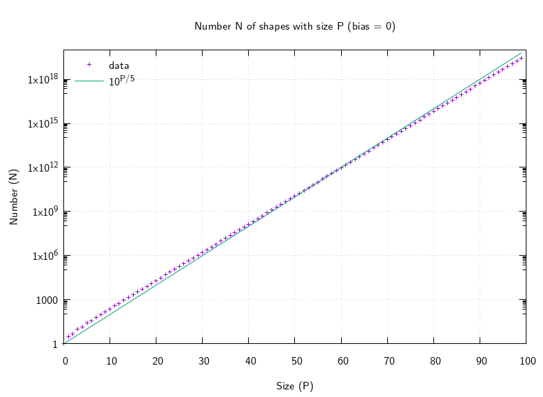
However, even with all these optimisations it's still really slow, because it takes time at least the order of the output count (because it is only incremented by 1 each time), and the output count grows rapidly. It took around 2 hours to calculate the first 45 terms. Just by counting lines as the number of digits increases, I could see that increasing the size by 5 multiplies the count by about 10, so the asymptotics are about O(10p/5). Here's a plot:
Two hours to calculate 45 terms is terrible, and I don't really need to calculate the actual shapes if I'm only interested in how many there are. So I started from scratch: how does the count change when you combine shapes. To do this I scribbled some diagrams, at first trying to combine two arbitrary shapes end-to-end, but that ended in failure. Success came when I considered the basic shape of length 2 (a single matrix) and considered what happens when appending an item. Then I made this work in reverse. Switching back to Haskell because it has good support for (unbounded) Integer, and good memoization libraries, I came up with this:
import Data.MemoTrie -- package MemoTrie on Hackage

-- count shapes of length n with p parameters that start with a and end with y
count = mup memo3 $ \n p a y -> case () of
  _ | n <= 1 || p <= 0 || a <= 0 || y <= 0 -> 0 -- too small
    | n == 2 && p /= a * y -> 0 -- singleton matrix mismatch
    | n == 2 && p == a * y -> 1 -- singleton matrix matches
    | otherwise -> -- take element y off the end leaving new end x
      sum [ count (n - 1) q a x
          | x <- [1 .. p]
          , let q = p - y * x
          , q > 0
          ]

total p = sum [ count n p a y | n <- [2.. p + 2], a <- [1 .. p], y <- [1 .. p] ]
This works so much faster, that 45 terms takes about 10 seconds using about 0.85 GB of RAM (and the results output are the same). Calculating just the 100th term (which is 28457095794860418935) took about 220 seconds using about 8.8 GB of RAM, but if you calculate terms in sequence the memoization means values calculated earlier can be reused, speeding the whole thing up: calculating the 101th term (which is 44259654087259419852) as well as the 100th term in one run of the program took about 260 seconds using about 16.4 GB of RAM. Calculating the first 100 terms in one run took about 390 seconds using about 20 GB of RAM.
Click to expand:A long-winded digression about fitting and residuals
without the images that would make it comprehensible - gnuplot crashed
before I could save them, losing its history in the process...
Using gnuplot I fit a straight line to the (natural) logarithm of the data points, which matched up pretty well, provided I skip the first few numbers (I'm only really interested in the asymptotics for large x so I think that's a perfectly reasonable thing to do):
gnuplot> fit [20:100] a*x+b "data.txt" using 0:(log($1)) via a, b
...
Final set of parameters            Asymptotic Standard Error
=======================            ==========================
a               = 0.441677         +/- 1.781e-06    (0.0004033%)
b               = 1.06893          +/- 0.0001137    (0.01064%)
...
gnuplot> print a
0.441677054485047
gnuplot> print b
1.0689289118356
Investigating the residuals showed an interesting pattern, they oscillate around zero getting smaller rapidly, until about x=35, after which they're all smaller than 0.000045. But then they are positive for a while and gradually decreasing to a minimum at x=73 or so, then the sign changes and they start increasing again. I thought with a better fit curve the oscillations would continue getting smaller, but I'm not sure how much more data I need. With the upper fit range limit set to 100, the asymptotic standard errors decrease by about a factor of 10 when I raise the lower fit range limit by 10. With the lower fit range limit set to 90, the earlier residuals are similar to those with the wider fit range limit, and the later residuals continue to oscillate getting smaller exponentially (magnitudes form a straight line on a graph with logarithmic scale).
gnuplot> fit [90:100] a*x+b "data.txt" using 0:(log($1)) via a, b
...
Final set of parameters            Asymptotic Standard Error
=======================            ==========================
a               = 0.441676         +/- 4.801e-12    (1.087e-09%)
b               = 1.06901          +/- 4.539e-10    (4.246e-08%)
...
gnuplot> print a
0.441675976841257
gnuplot> print b
1.0690075089073
Fitting a curve to the residuals seemed to improve things a bit, the final form of the function I came up with was something like:
\[ \exp(a p + b + (-1)^p \exp(c p + d)) \]
with a and b as above and
c = -0.246716071616843
d = -1.18363693943899
The residuals of that with the data show no simple pattern - there is some low frequency oscillation at the left end? Not sure. I still don't really know enough statistics to analyze this kind of thing.
Moving back to the original problem, neural networks often have a bias term. This means an extra element that is always 1 is appended to the input vector of each stage, but not the output. This means that for example the matrices in the shape [a,b,c] would have dimensions (a+1)×b and (b+1)×c, instead of a×b and b×c without bias.
In Haskell one would calculate
sum (zipWith (*) (map (+ 1) s) (tail s)), even though the
naive Haskell is slow I did it to get the first few terms for validation
purposes. I added it to the C version, and got some more terms, and
finally updated the fast Haskell version. Here are the first few terms
as calculated by naive Haskell before it ran out of memory:
0, 1, 1, 3, 2, 6, 5, 9
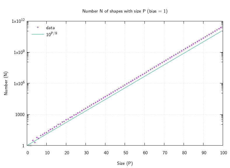
which match those calculated by C which isn't terribly slow here, at least to start with, because the growth of the output is much less rapid, more like O(10p/9):
The fast (memoizing) Haskell took about 420 seconds to calculate the first 100 terms using about 19.7 GB of RAM. It took about 17 seconds to calculate the first 50 terms using about 0.82 GB of RAM. The C took about 15 seconds (slightly faster) to calculate the first 50 terms, using less than about 1.4 MB of RAM (almost nothing in comparison). The 50th term is 538759 (both programs match), the 100th term is 240740950572. The C slows down by at least the size of the output, which is exponential in the input, so I didn't wait to see how long it would take to calculate 100 terms.
Here you can download the code for these experiments, and the output data tables:
- Makefile
- exhaustive.hs slow Haskell that exhausts RAM
- pruning.c slow C that needs almost no RAM
- memoizing.hs fast Haskell that needs lots of RAM
- unbiased.txt 100 terms starting 1, 3, 5, 10, ... (bias = 0)
- biased.txt 100 terms starting 0, 1, 1, 3, ... (bias = 1)
- plots.gnuplot source code for plots
- unbiased.png logarithmic plot (100 terms, bias = 0)
- biased.png logarithmic plot (100 terms, bias = 1)