Approximating cosine
EDIT there is another post with an update
The problem
Mathematical functions like \(\cos()\) can be expensive to evaluate accurately. Sometimes high precision isn't necessary, and a cheap to compute approximation will do just as well.
Symmetry and range reduction
The cosine function oscillates smoothly between \(1\) and \(-1\). It is even:
\[ \cos(-x) = \cos(x) \]
It also has another symmetry:
\[ \cos(\pi - x) = -\cos(x) \]
And it is periodic:
\[ \cos(x + 2 \pi) = \cos(x) \]
Irrational numbers like \(\pi\) are a pain for computers, so for ease of implementation we'll define a \(\cos\) variant that has a period of \(1\) instead of \(2 \pi\).
Due to the symmetries it's only necessary to approximate \(1/4\) of the waveform. The cosine is closely related to the sine, they are out of phase by \(\pi/2\):
\[ \sin(x + \pi/2) = \cos(x) \]
Given an \(x\), first make it positive (using the evenness of \(\cos\)):
\[ x \gets |x| \]
Then reduce it into the range \([0..1]\) by keeping the fractional part (using the periodicity of our modified \(\cos\)):
\[ x \gets x - \operatorname{floor}{x} \]
Now we can fold over the symmetry line at \(1/2\) (originally \(\pi\)):
\[ x \gets |x - 1/2| \]
Our \(x\) is now in \([0..1/2]\), and its cosine should be \(-1\) at \(x = 0\) and \(1\) at \(x = 1/2\). The halves are a bit awkward, it'd be nicer if the cosine was \(-1\) at \(x = -1\) and \(1\) at \(x = 1\). So:
\[ x \gets 4 x - 1 \]
The prevoius steps could be combined into one, as in the C99 source code file cosf9.h, at the start of the function cosf9_unsafe():
\[ x \gets |4 x - 2| - 1 \]
Polynomial approximation
We now have \(x\) in \([-1..1]\) and the desired cosine of the original value in the same range. The symmetries of cosine mean we have an odd function now, with:
\[ f(-x) = -f(x) \]
A polynomial is a sum of powers of a variable, and it's fairly obvious that an odd polynomial can have only odd powers. Let's write
\[ f(x) = a x + b x^3 + c x^5 + d x^7 + \ldots \]
Which are the best values of \(a, b, c, d, \ldots\) to pick to best approximate the desired function? Given that it's odd, it's pointless to consider both positive and negative inputs (or zero), so positive it is. We know that \(f(1) = 1\), which gives the contraint:
\[ 1 = a + b + c + d + \ldots \]
If the function \(f\) matches the desired curve, then its slope will match too. The derivative of \(\sin\) is \(\cos\), and of \(\cos\) is \(-\sin\), and of the power \(x^n\) is \(n x^{n-1}\). Our function \(f\) happens to be \(\sin(x \pi / 2)\) (exercise: demonstrate it), and by the chain rule and linearity of differentiation its derivative at \(0\) is \(\pi/2\). So we get another constraint:
\[ \pi/2 = a \]
That's an easy one to solve! The derivative at \(1\) is \(0\) (the top of the waveform cycle is instantaneously horizontal), whcih gives:
\[ 0 = a + 3 b + 5 c + 7 d + \ldots \]
So far so good, but we have 3 linear equations and 4 unknowns, so there's not enough information to find a unique solution. The second derivative at \(1\) should be \(\pi^2/4\), so our final equation can be:
\[ \frac{\pi^2}{4} = 6 b + 20 c + 42 d + \ldots \]
Putting into matrix form:
\[ \begin{pmatrix} 1 & 1 & 1 & 1 \\ 1 & 0 & 0 & 0 \\ 1 & 3 & 5 & 7 \\ 0 & 6 & 20 & 42 \end{pmatrix} \begin{pmatrix} a \\ b \\ c \\ d \end{pmatrix} = \begin{pmatrix} 1 \\ \frac{\pi}{2} \\ 0 \\ \frac{\pi^2}{4} \end{pmatrix} \]
Luckily there are plenty of software packages for solving matrix equations, I used GNU Octave (see the source code file cosf7.m, which solves a \(3 \times 3\) system with \(a = \pi/2\) already substituted). The answer that Octave gives is this:
\[ \begin{pmatrix} a \\ b \\ c \\ d \end{pmatrix} = \begin{pmatrix} + 1.5707963267948965580 \times 10^{+00} \\ - 6.4581411791873211126 \times 10^{-01} \\ + 7.9239255452774770561 \times 10^{-02} \\ - 4.2214643289391062808 \times 10^{-03} \end{pmatrix} \]
Quality
Now we have an approximation. But we don't know how good it is. A quick visual check is to plot the difference between our function and the the high quality cos() in the standard C maths library. But without a frame of reference, the numbers aren't necessarily all that meaningful.
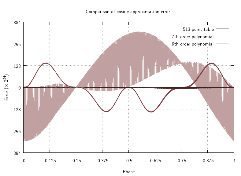
The music software Pure-data contains its own approximation of the cosine function, using an entirely different technique: linearly interpolated table lookup. Plotting the error in its approximation on the same scale as our function reveals a pleasant surprise: our order 7 polynomial's error deviates from the \(0\) axis (perfection) much less wildly than Pd's. But the deviation has a different character, Pd's is wildly swinging with a low frequency component, while ours has a hump. In the context of audio, these different variations might change the perception of the error (exercise: try double-blind listening tests to see which form is most obnoxious).
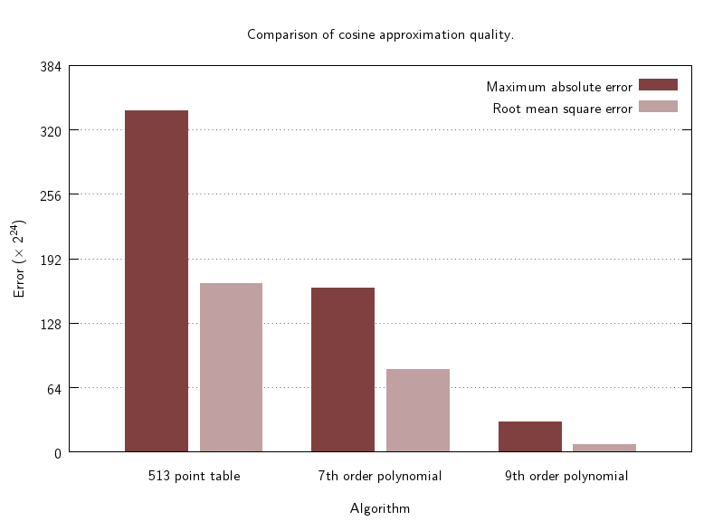
We can quantify the error in (at least) two ways, one is the maximum absolute deviation from perfection, and another is the root mean square (RMS) error, calculated by averaging the squares of the errors before taking the square root. Taking \(2^{30}\) randomly distributed phases and accumulating their error shows that the 7th order polynomial has about half the error as Pd's table look up, in both measures.
To gain higher quality (lower error statistics), we can increase the order of the polynomial, by adding an extra \(e x^9\). We need another constraint to be able to solve the equations, and a reasonable choice seems to be to pick the worst phase (around \(2/\pi\)) on the 7th order polynomial and force it to be exact. This gives:
\[ \sin(1) = \frac{2}{\pi} a + (\frac{2}{\pi})^3 b + (\frac{2}{\pi})^5 c + (\frac{2}{\pi})^7 d + (\frac{2}{\pi})^9 e \]
and we can solve the new \(5 \times 5\) matrix equation to get different values for all the coefficients. See the GNU Octave source code file cosf9.m for details, and the C source code file cosf9.h for the coefficients.
The 9th order polynomial is about five times more accurate than the 7th order polynomial, getting close to the limits of the 24bit mantissa of single precision floating point.
Speed
It's no point having a superb approximation if it's not faster than the full precision version, so benchmarking and optimisation is the final part of the evaluation (but any changes to the code in the hope of making it faster might have an impact on the quality, in sometimes unexpected ways - so check the metrics and graphs on each change).
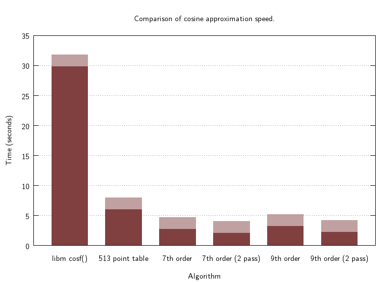
Unsurpisingly, the math library cos() is very slow, and the Pd cosine table is several times faster. But our polynomial approximations are faster still, with the 9th order not lagging far behind the 7th order. This took some effort, however. Putting too much into one inner loop puts pressure on the hardware, and performance can suffer. Something as counterintuitive as making two passes over the data, performing range reduction in the first pass and evaluating the polynomial in the second pass, can make a significant difference. Also important is splitting into smaller functions - with a smaller scope, the compiler can do a better job of making it go really fast.
The first version (not shown in the graphs) was somewhat disappointing - adding range reduction around the polynomial evaluation (which was already fast enough) made it seven times slower, slower than Pd's table implementation. Splitting it into two passes solved that problem, and then it turned out that with the functions split neatly, a single pass could now do nearly as well as two. See the source code file cosf9slow.h to see what it was like before the changes.
Conclusion
A 9th order polynomial approximation to the cosine function is about ten times faster than the accurate math library implementation, and about three times faster than linearly interpolated table lookup. Moreover the polynomial is over ten times more accurate than the table version.
The source code for this post is available at approximations on code.mathr.co.uk.
Thanks to the folks in the #numerical-haskell IRC channel for enlightening me about TLB pressure, even though no Haskell was involved.