mathr / blog / #

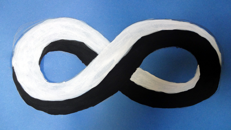
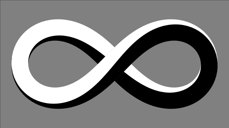
I painted the above in acrylic yesterday, today I digitally recreated it:

The basic shape is the lemniscate of Bernoulli, which has the parametric equation:

\[\begin{aligned} x &= \frac{\cos t}{\sin^2 t + 1} \\ y &= \frac{\cos t \sin t}{\sin^2 t + 1} \\ z &= \frac{\sin t}{2} \end{aligned}\]

I added the third \(z\) coordinate to avoid self-intersection in 3D, the real lemniscate is 2D. The lemniscate is a curve with no width, but the painting represents it using a square cross-section, with a half-twist each time around the loop.

A Möbius strip is a 2D surface of a loop with a half-twist, the real strip has no thickness, but the painting represents it using a square cross section, as if the two sides (which are really the same side!) of the surface were pushed apart, and the single boundary of the strip now becomes a surface, which happens to be another Möbius strip with its surface pushed apart.

Thickening the 1D lemniscate in 3D space to a 2D surface surrounding a square cross section with a half-twist involves some slightly fiddly maths. The steps involve finding a local coordinate frame (an orthonormal basis, three mutuallly perpendicular unit-length vectors) along the curve, applying the twist normal to the curve, and then using the twisted local coordinate frame to generate the square cross section.

The local coordinate frame has one basis vector in the direction of the curve. This can be found by differentiation with respect to \(t\) followed by normalization. The parametric equations are a bit awkward to differentiate by hand, but the free computer algebra software Maxima can perform symbolic differentiation:

(%i1) diff( cos(t)/(sin(t)^2 + 1) , t );
                                            2
                           sin(t)      2 cos (t) sin(t)
(%o1)                  - ----------- - ----------------
                            2               2        2
                         sin (t) + 1    (sin (t) + 1)
(%i2) diff( cos(t)*sin(t)/(sin(t)^2 + 1) , t );
                       2             2             2       2
                    sin (t)       cos (t)     2 cos (t) sin (t)
(%o2)           - ----------- + ----------- - -----------------
                     2             2               2        2
                  sin (t) + 1   sin (t) + 1    (sin (t) + 1)
(%i3) diff( sin(t)/2 , t );
                                    cos(t)
(%o3)                               ------
                                      2

This vector needs to be normalized for the basis, so divide each coordinate by the length of the vector (which is the square root of the sum of the squares of the coordinates, by Pythagoras' theorem).

Having one basis vector (call it \(\mathbf{u}\)) is a start, but there are two more to find. The vector cross product of two vectors gives a third vector orthogonal to both, so picking an arbitrary direction as the \(z\) axis \((0, 0, 1)^T\), the second basis vector is in the direction \(\mathbf{z} \times \mathbf{u}\), call it \(\mathbf{v}\) when normalized. The third and final basis vector can now be found: \(\mathbf{w} = \mathbf{v} \times \mathbf{u}\). This doesn't really need normalization because the arguments are orthonormal, but rounding errors might make it useful to renormalize anyway.

To give a half twist around the loop, the basis vectors need to be rotated around the curve - having picked one basis vector as the curve direction, the task reduces to a simple planar rotation, whose matrix is:

\[\begin{aligned} M &= \begin{pmatrix} 1 & 0 & 0 \\ 0 & \cos \theta & \sin \theta \\ 0 & -\sin \theta & \cos \theta \end{pmatrix} \\ \theta & = \frac{t}{2} + \frac{\pi}{4} \end{aligned}\]

The \(\frac{\pi}{4}\) phase offset is to make the ends of the loops flat. Now the curves along the corners of the square cross-section can be defined in terms of the transformed basis vectors, and the two flat surfaces (one white and the other black) are formed by interpolating between neighbouring curves. In the source code linked below the transformed basis vectors are called \(p\) and \(q\) and the edge curves are called \(i_1\), \(j_1\), \(i_2\) and \(j_2\), with the surfaces \(k_1\) and \(k_2\).

I used gnuplot for the visualization, it's a bit awkward having to separate out the vector components, and having to dump the parametric data to table files and replot them to be able to set the fill colour is even more awkward. But it did the trick, here's the source for the image: moebius_infinity.gnuplot.

Exercise 1: adjust the thickness of the square cross-section to better match the original painting.

Exercise 2: generate an animation of the loop twisting, by rendering frames with different \(\theta\) phase offsets.

Exercise 3: try a loop with a quarter twist, using a rainbow colour gradient that wraps around the loop just once.

Exercise 4: try different cross-sections: for example a triangle or pentagon.